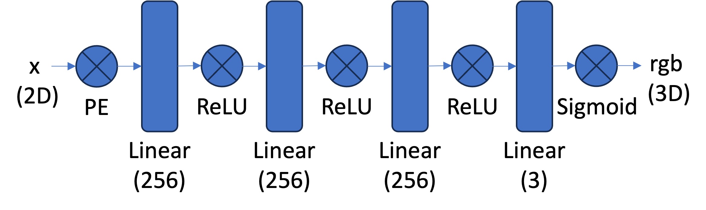
MLP model architecture
First, we create a multilayer perceptron network with sinusoidal positional encoding. This network will take in the 2d pixel coordinates and will output the 3D pixel colors.
The next step is to implment a Dataloader that randomly samples pixels from the image at each iteration. This is done because selecting all the pixels from a high resolution image would exceed the GPU memory limit.
As suggested, I used MSE error as the loss function of the difference between predicted pixel value and true color. Using this, I trained my networks using Adam for 2000 iterations.
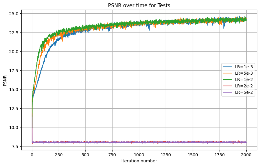
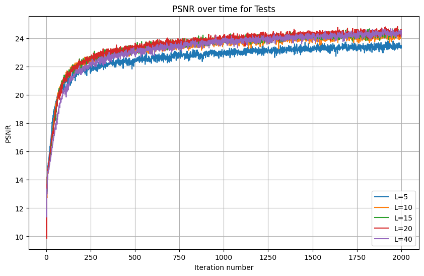
The next step is hyperparameter tuning. I chose to explore the impact of varying learning rate and L. Here are my results:
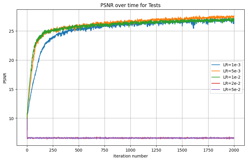
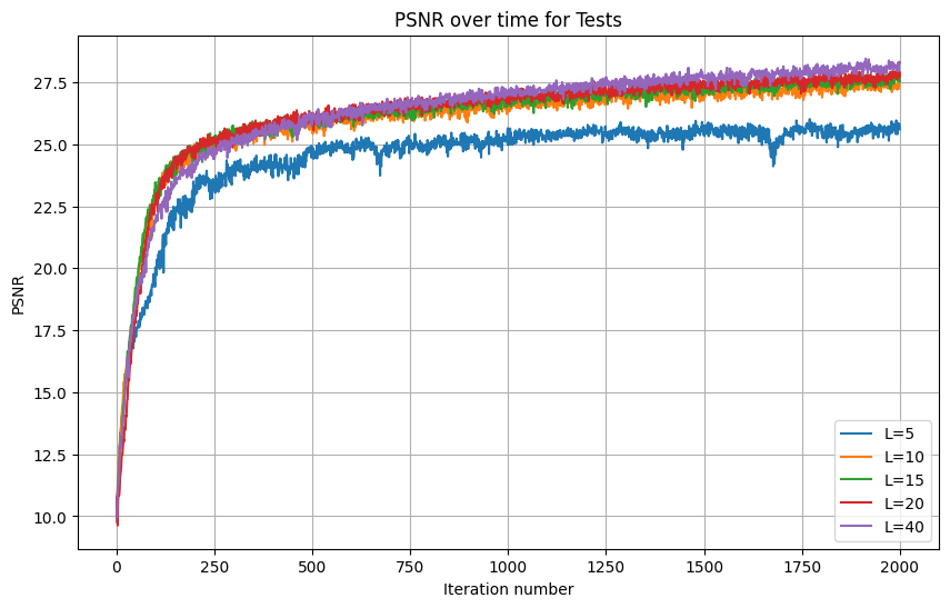
As can be seen from the graph, the optimal learning rate out of those I tested was 5e-3. Also, we can see that larger Ls lead to better results over 2000 iterations. However, there isn't much difference when L surpasses 10. For that reason, I used 5e-3, but kept the recommended L=10.
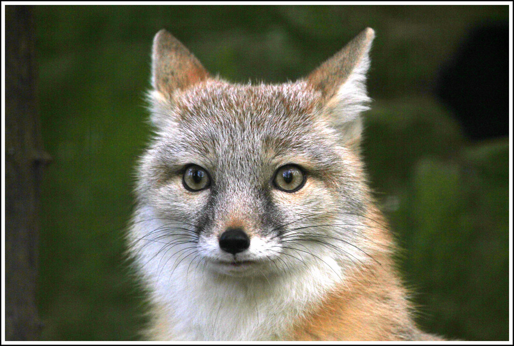
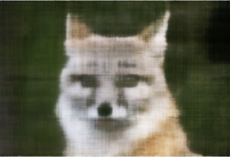
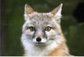
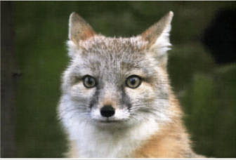
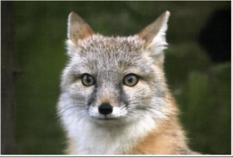
The first image I used it this photo of a fox:
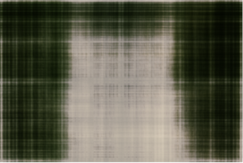
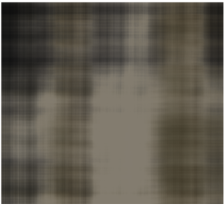
With the selected parameters, I obtained the following results:

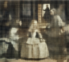
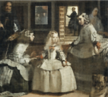
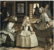
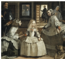
Then, I repeated the process with the 'Las Meninas' painting. I chose this because there isn't a single subject in the middle but rather multiple characters. Like with the fox image, the first step was hyperparameter tuning:
Interestingly, in this painting (and over 2000 iterations), there was no perceptible difference between learning rates, so long as they were lower than 2e-2. I chose the highest learning rate out of the ties since it had better results at earlier iterations. As for L tuning, there was no perceptible difference for L above 10. Here are my resulting images at various iterations:

In the second part of the project, I use a Neural Radiance Field to represent 3D space. Compared to the original NERF paper, we will user lower resolution images and preprocessed cameras. Still our overall procedure is similar.
This formula relates camera coordinates to world coordinates:
\[ \begin{bmatrix} x_c \\ y_c \\ z_c \\ 1 \end{bmatrix} = \begin{bmatrix} \mathbf{R}_{3 \times 3} & \mathbf{t} \\ \mathbf{0}_{1 \times 3} & 1 \end{bmatrix} \begin{bmatrix} x_w \\ y_w \\ z_w \\ 1 \end{bmatrix} \]
The matrix to the right of the equals sign is the extrinsic (w2c) matrix. This relates the world coordinates to the camera coordinates. Next we relate the camera coordinates to the pixel coordinates using the following equations:
Pixel to Camera: \[ s \begin{bmatrix} u \\ v \\ 1 \end{bmatrix} = \begin{bmatrix} f_x & 0 & o_x \\ 0 & f_y & o_y \\ 0 & 0 & 1 \end{bmatrix} \begin{bmatrix} x_c \\ y_c \\ z_c \end{bmatrix} \]
With these two conversions, we only need to define a pixel to ray conversion, to obtain ray origin and direction.
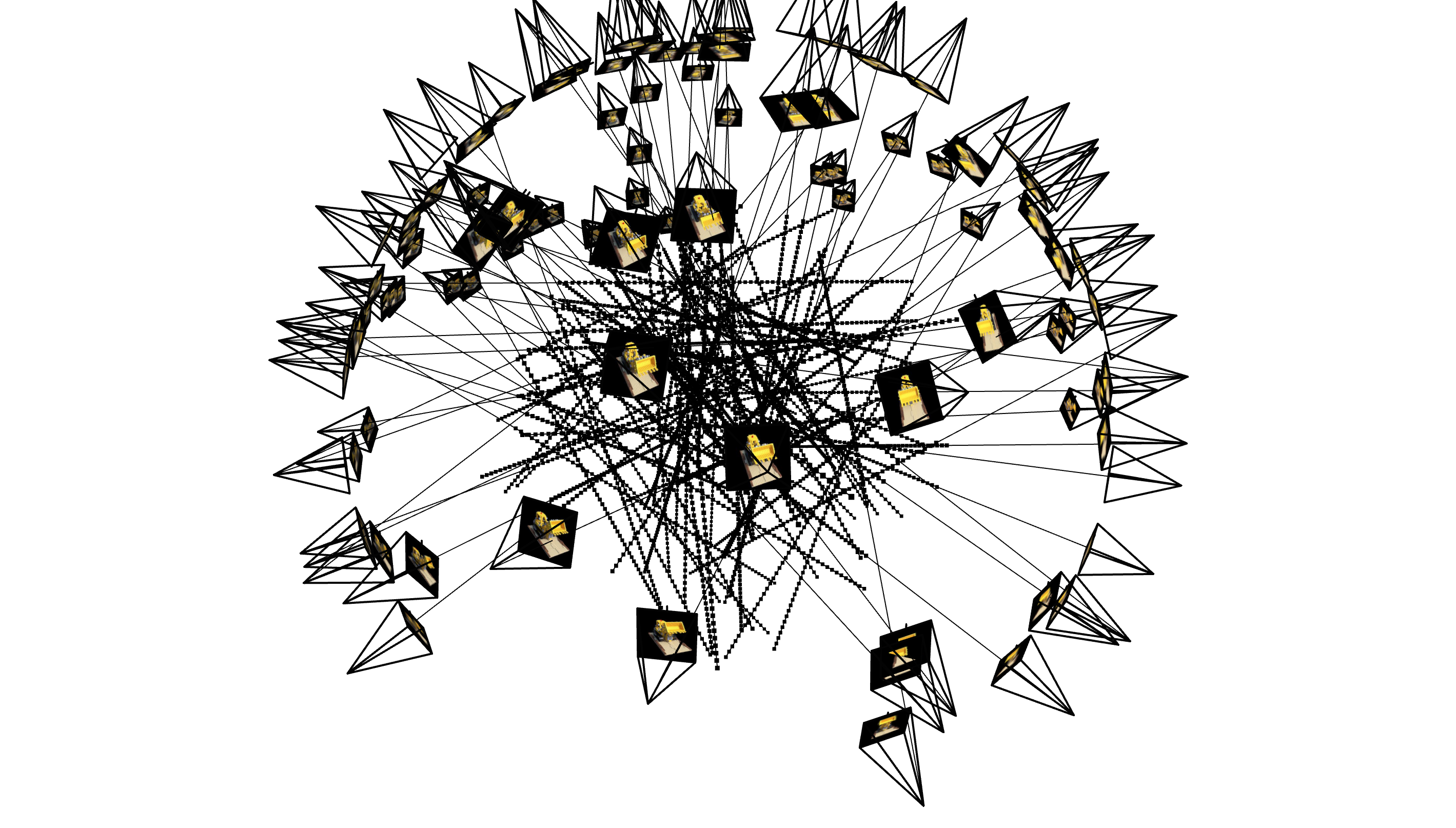
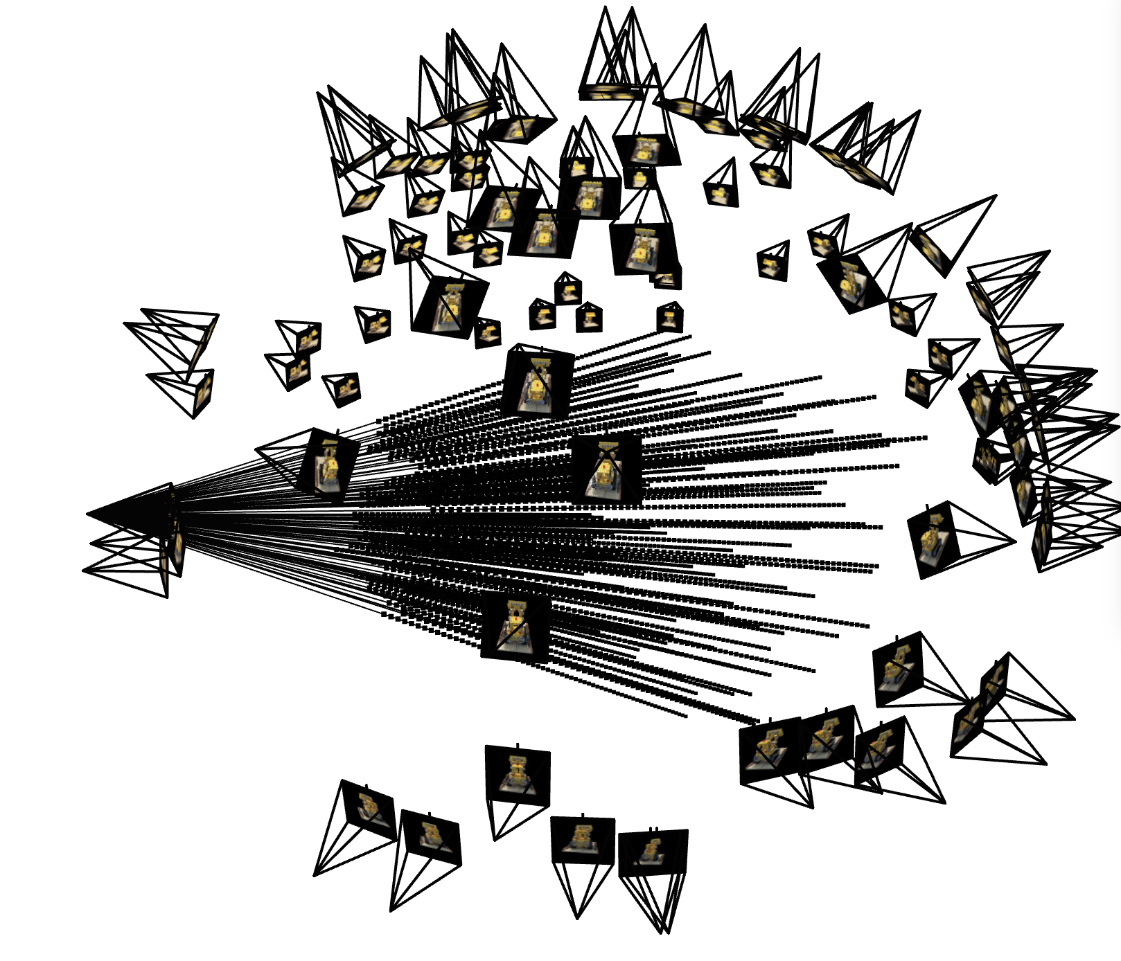
Using the ray creation that I implemented for part 2.1, we may now implement sampling. The task becomes harder than it was for the 2D Case. Now, we must first sample rays from images and then sample points from rays.
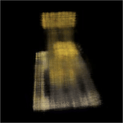
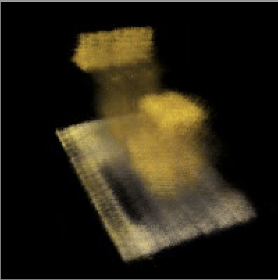
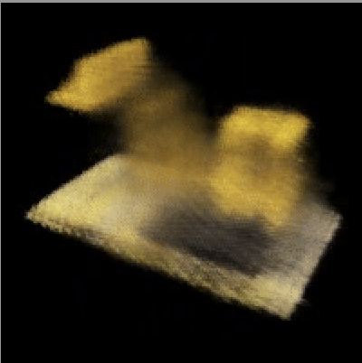
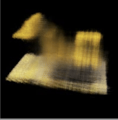
We may use the provided visualization to check that the code is so far correct. Here are the results I obtained:
Here is the structure of a Neural Radiance Field:
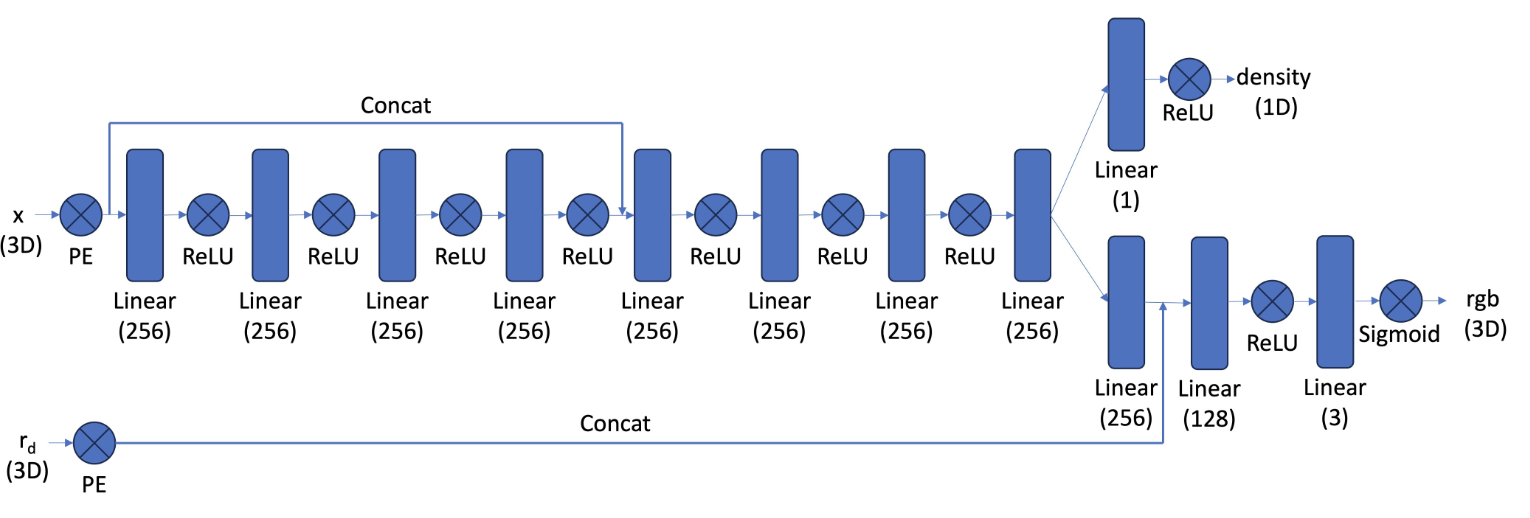
As part of this section, I implemented the network shown. Compared to the network that I used in part A, the first observation that one can make is that the net is significantly deeper. This can be easily explained by the fact that 3D is way more challenging than 2D. It also stands out that we use an adapted version of a positional encoding, that now encapsulates both coordinates and ray direction.
\[ \hat{C}(\mathbf{r}) = \sum_{i=1}^{N} T_i \left(1 - \exp(-\sigma_i \delta_i)\right) \mathbf{c}_i, \quad \text{where} \quad T_i = \exp\left(-\sum_{j=1}^{i-1} \sigma_j \delta_j\right) \]
With this defined, we're ready to train the model and evaluate our results. Here is the validation accuracy of the model:
.png)
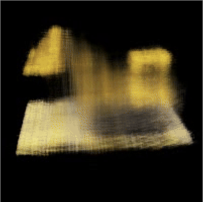
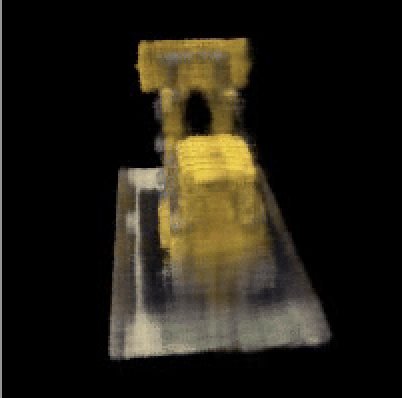
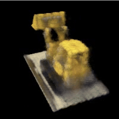
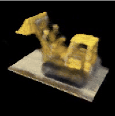
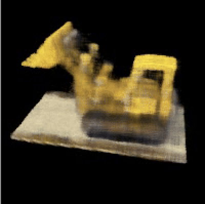
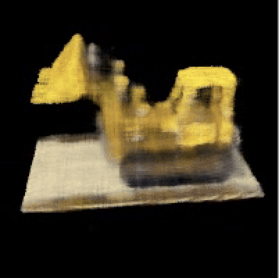
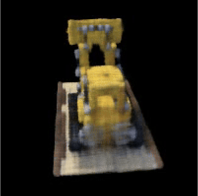
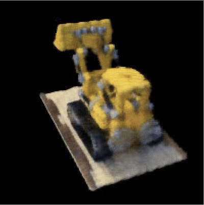
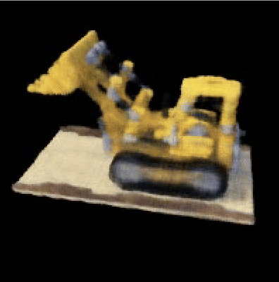
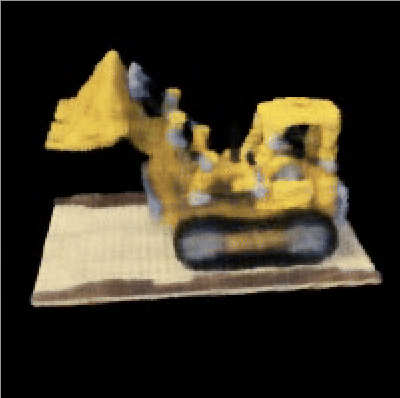
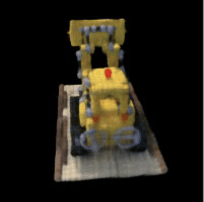
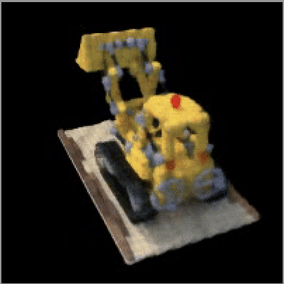
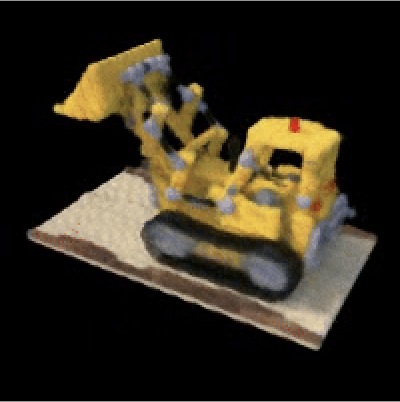
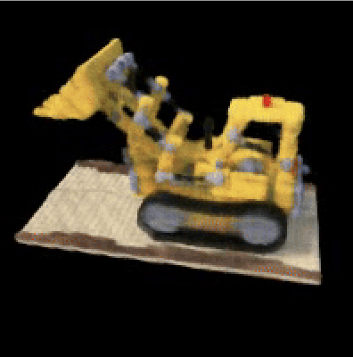
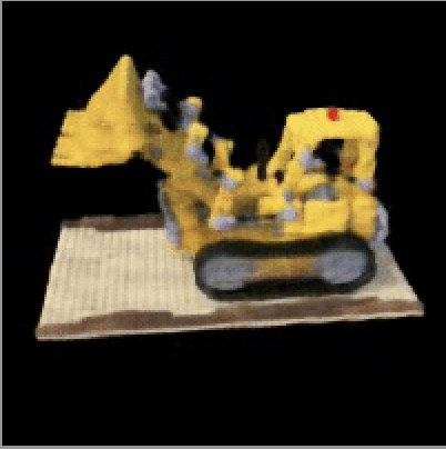
Instead of comparing results for 6 still images, I decided that it looked better to create the video visualization for intermediate models too (in effect comparing 60 frames). I've also included the first six frames of each in the appendix to ensure that I meet the requirement.
For the bells and whistles portion, I decided to change the background color. This can be done with the same trained version of the model. This is possible because we trained our model to identify rays where there is no object. At these points, we should inject backgound color. Therefore, by adding the product of accumulated transmittance and our desired RGB background we can create a non-black setting for our Lego. Here are a grey and red background:
Here are the first 6 frames of the result gif, in case the grader is looking at the pdf version: