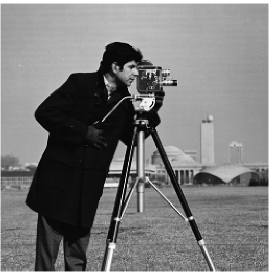
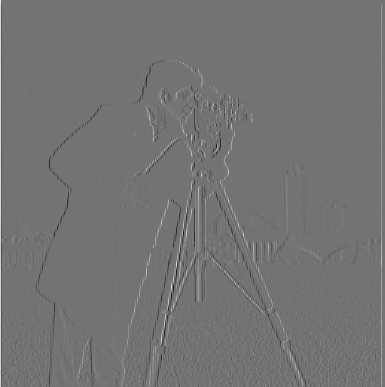
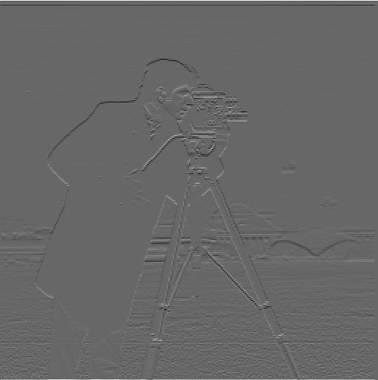
In this section, we use the finite difference operators to obtain the partial derivatives of an image with respect to the x and y directions. To do this, we convolve the image with the vector [1 -1] (for dx) and [1 1].T (for dy). Here are the results:


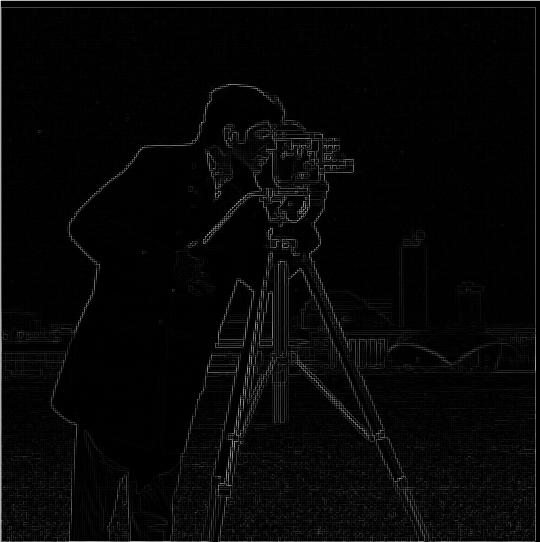
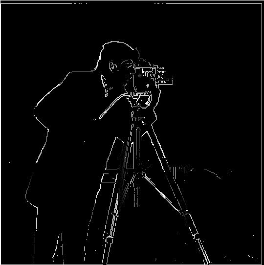
As part of this section, I also computed the gradient magnitude image and binarized to create an edge image. The gradient magintude image like the gradient of any other 2-dimensional function f(x,y). That is, grad = sqrt((dI/dx)^2+(dI/dy)^2). To create the gradient image, we simply calculate this value at each point of the original image. An inperfection of the binarized image is that it's very noisy because we had to pick a large threshold. We'll solve this in the following section.
Since the above image was very noisy, we will apply a gaussian filter before calculating the gradient image. That is, we first blur the image and then compute gradient magnitude:
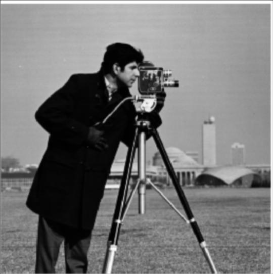
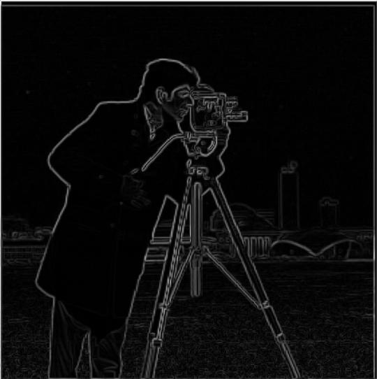

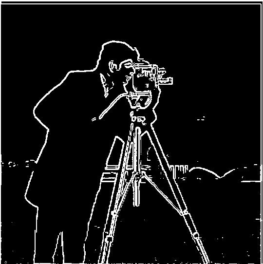
In the case of the new edge image, we can see that it's significantly less noisy, because we were able to choose a much lower binary threshold (namely, I picked .08 instead of 0.3). Given that we blurred the image first, random noise won't make this threshold, leading to better results.
As prompted, I also carried out this procedure by calculating first the DoG filters (for x and y), and applying those analogously to part a. Indeed, we obtain the same result:


In this section, I explored how amplifying the higher frequencies of an image led to the image appearing "sharper". Indeed, to obtain a high pass filter, we subtract a low-pass filter from them image. Then, we add the high-filtered image to the original using some scaling factor alpha and observe the results. For this section, I picked old image that were originally not "sharp". I display the sharpened verisons for different values of alpha - my favorite is the berlin wall picture.
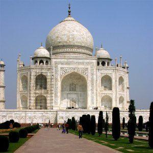
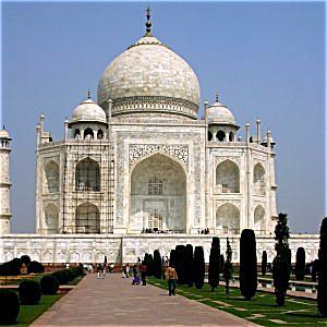
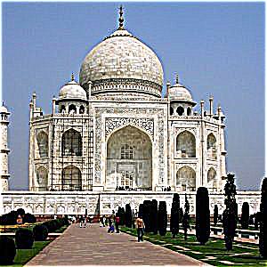
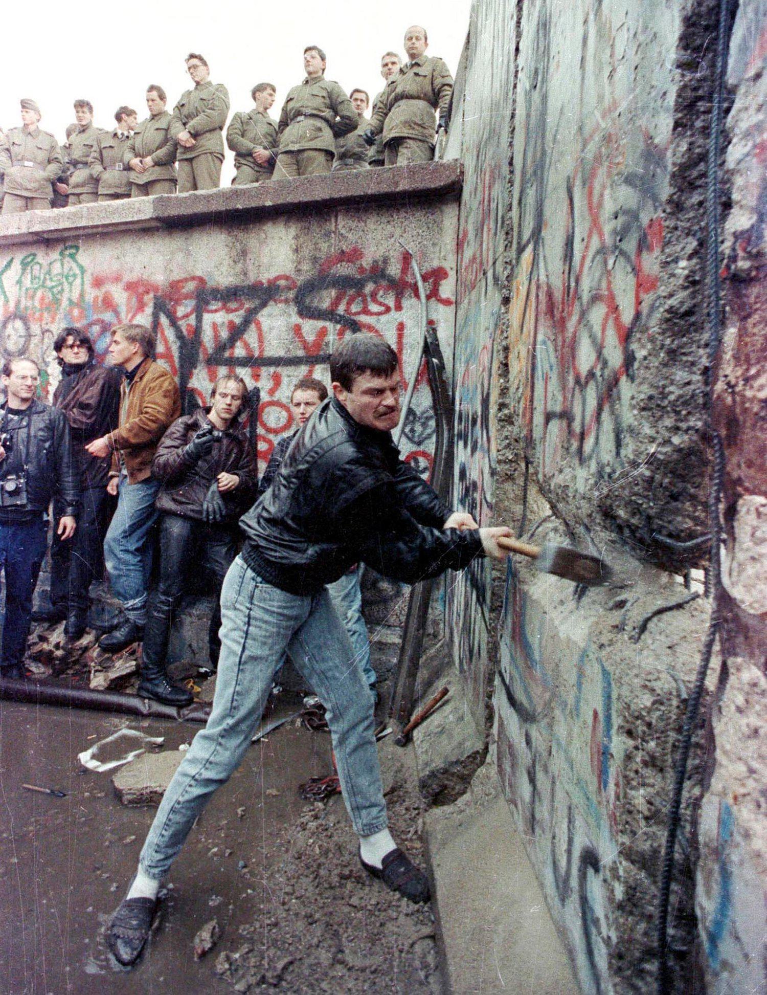

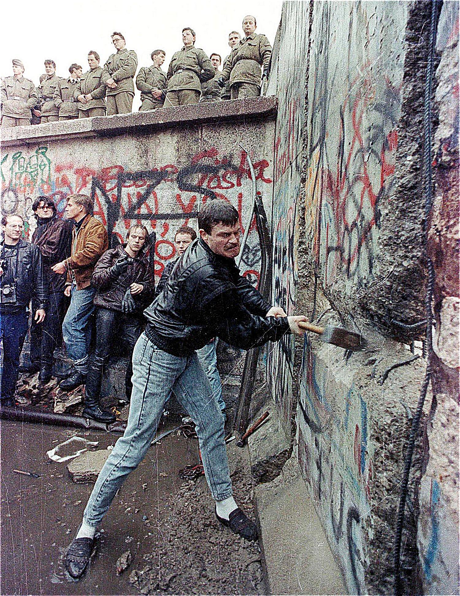
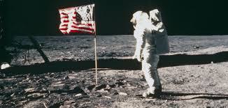
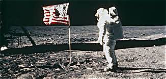
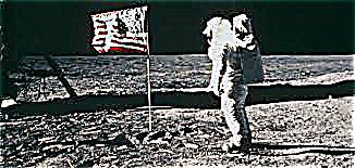
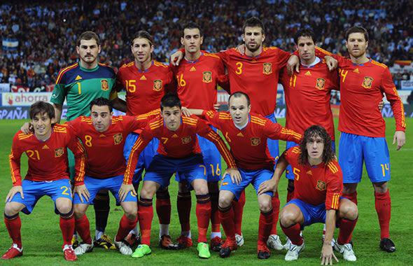
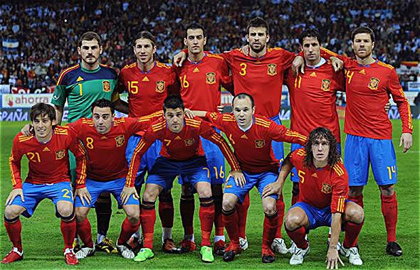
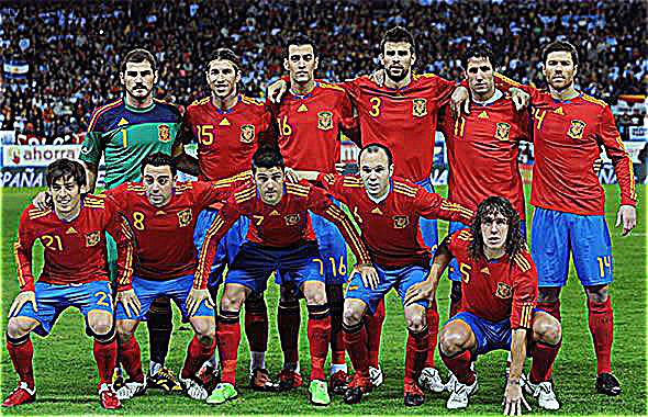
As we can see the optimal alpha isn't constant but rather depends on the original image. A value of alpha that is too large results in noise being amplified to the point where the image becomes worse. For example, the football squad image looks better at alpha=1 than 4.
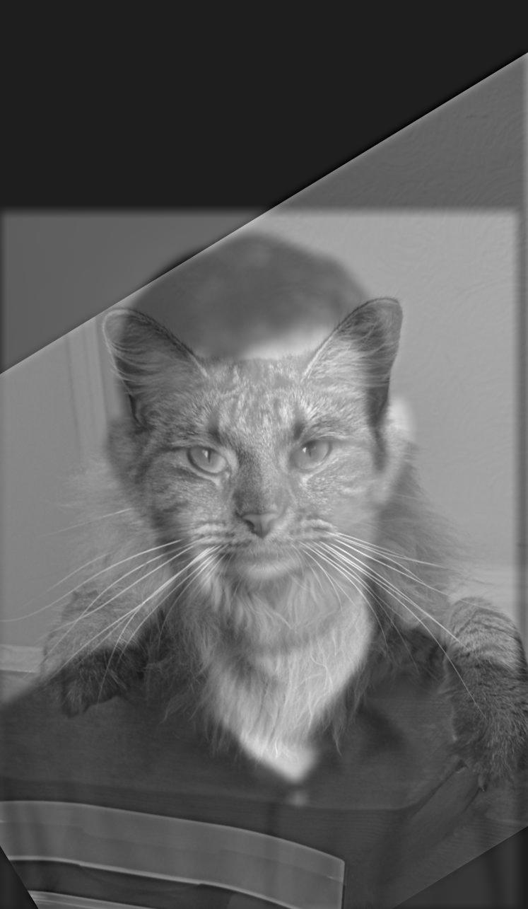
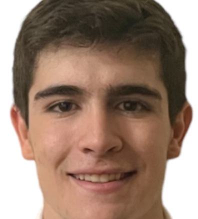
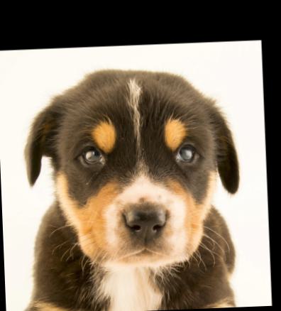
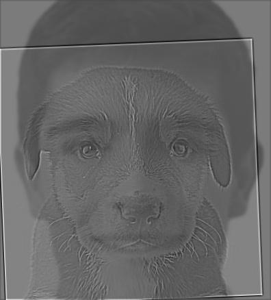


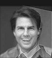
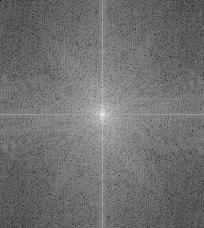
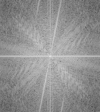
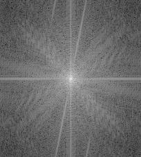
For my favorite example (the Tom Cruise happy/sad), here are the log magnitudes of the fourier transforms:
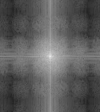
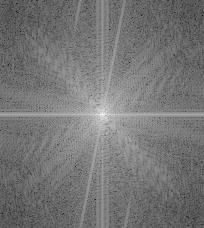

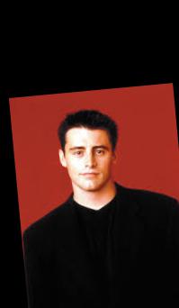
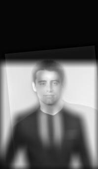
Here is an example that didn't work: I tried to join Barney Stinson and Joey Tribbiani's faces into one but couldn't. Due to the relative size of their faces and the specific picture I chose, only Joey is visible at any distance:

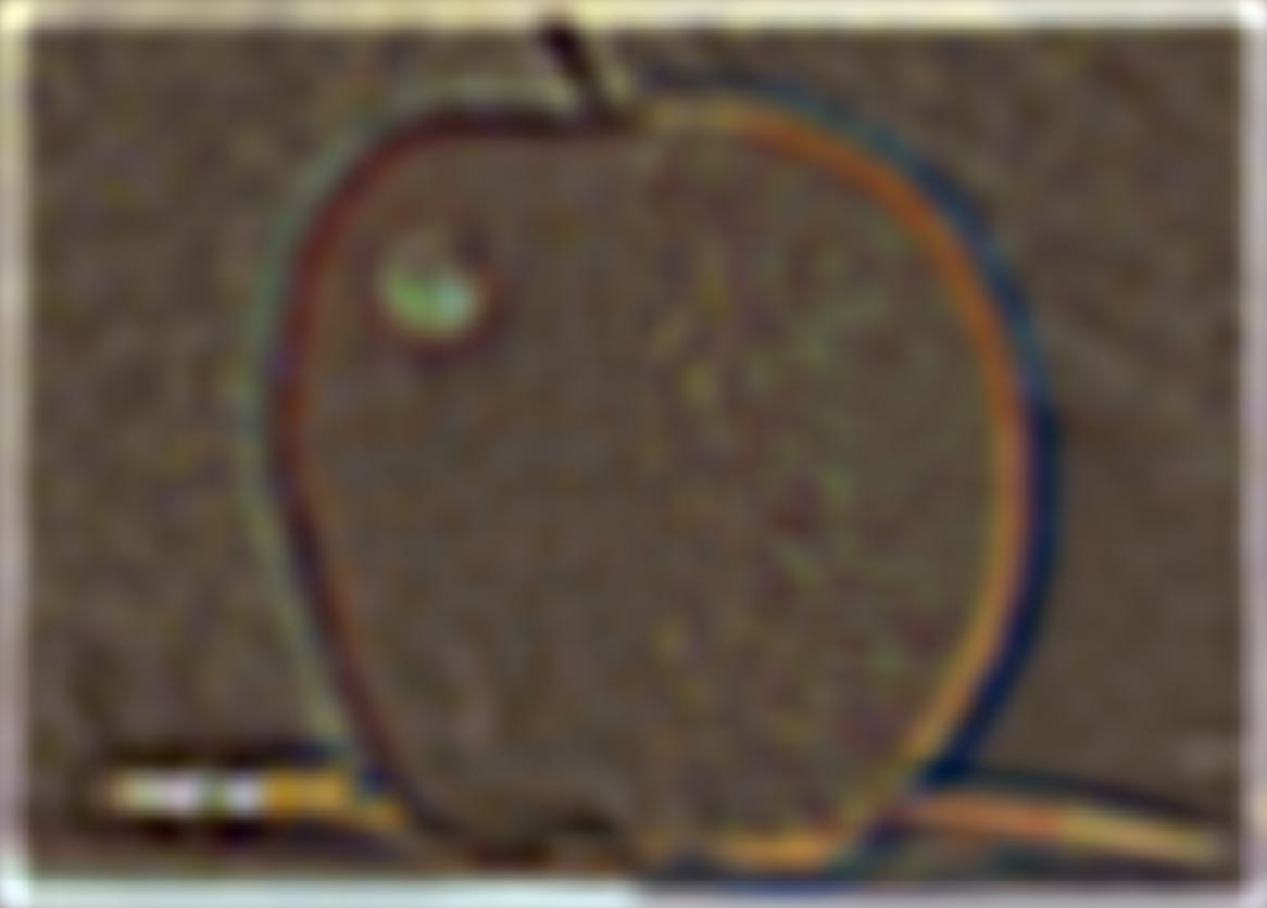
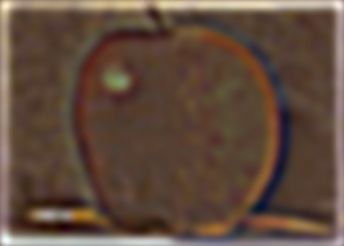
A gaussian stack is an image to which we apply a gaussian filter repeatedly. That is G_n = I*G^n. The laplacian filter is calculated by subtracting an element from the gaussian Stack from the next. That is L_n = G_n - G_(n+1). The following are the gaussian and laplacian stacks for oraple apple:

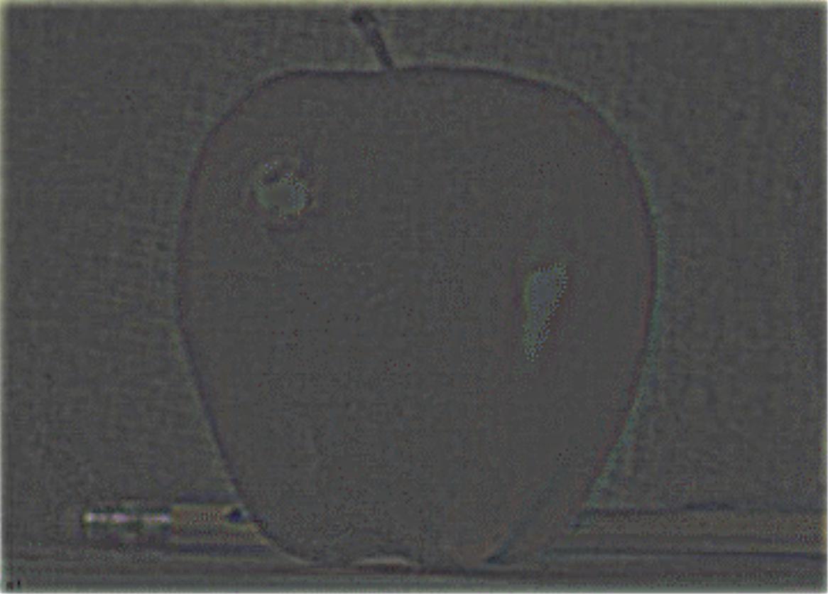
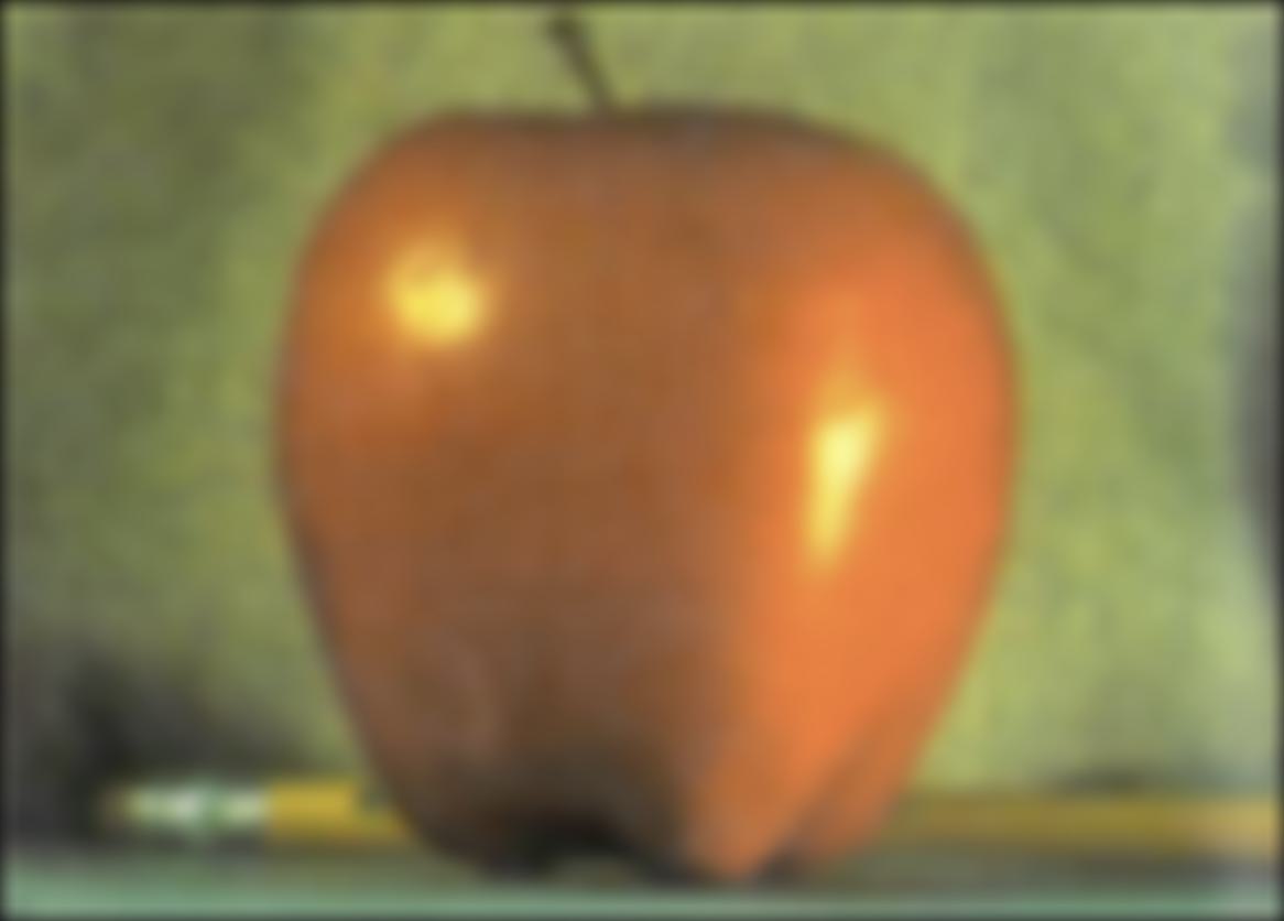
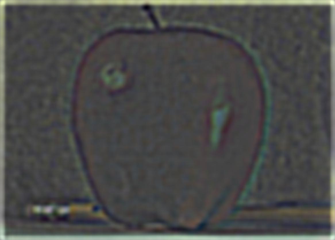
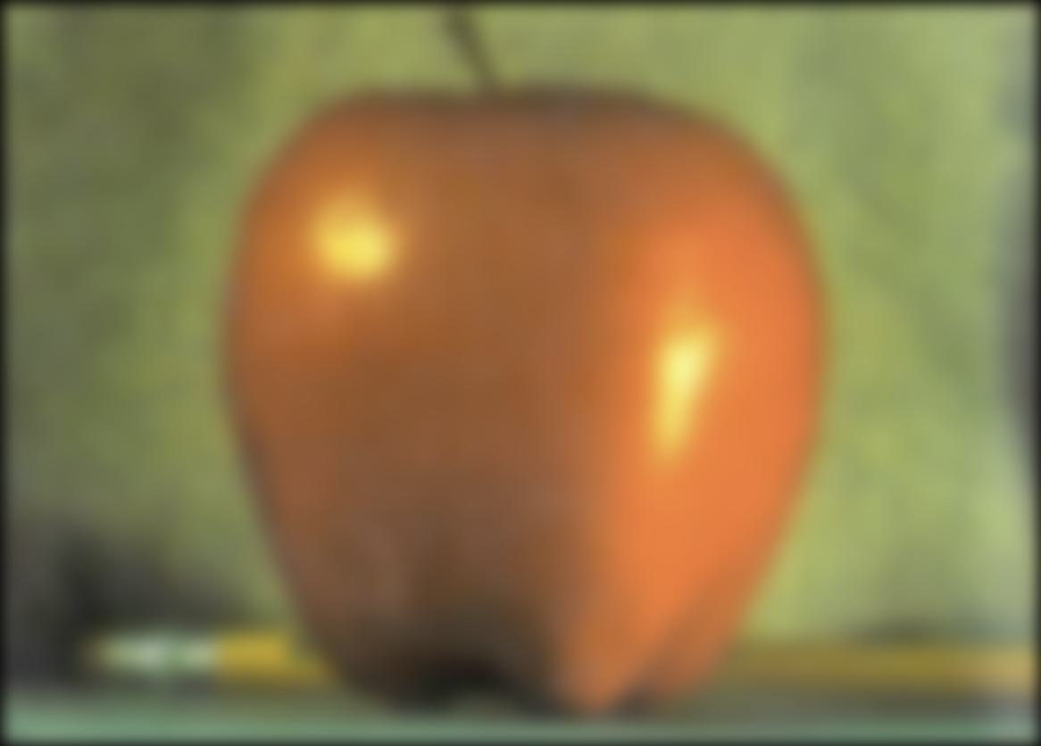
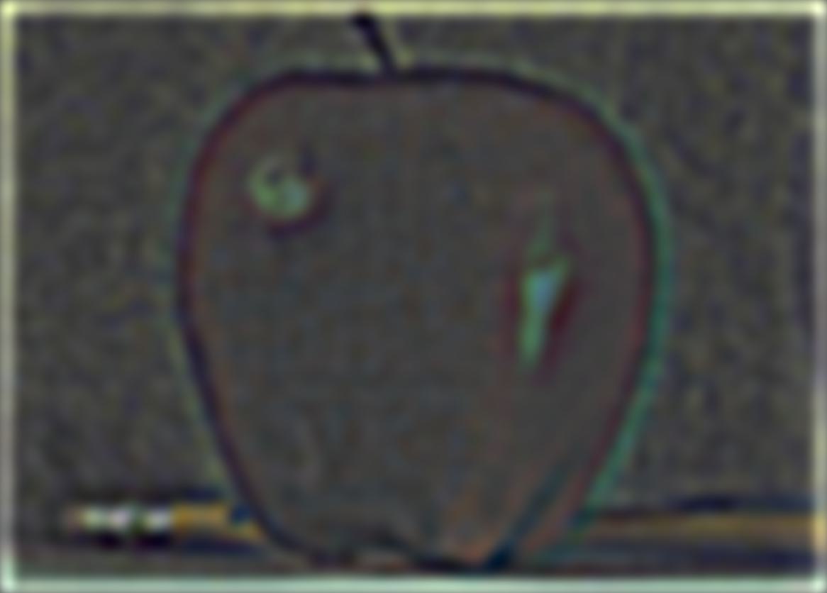
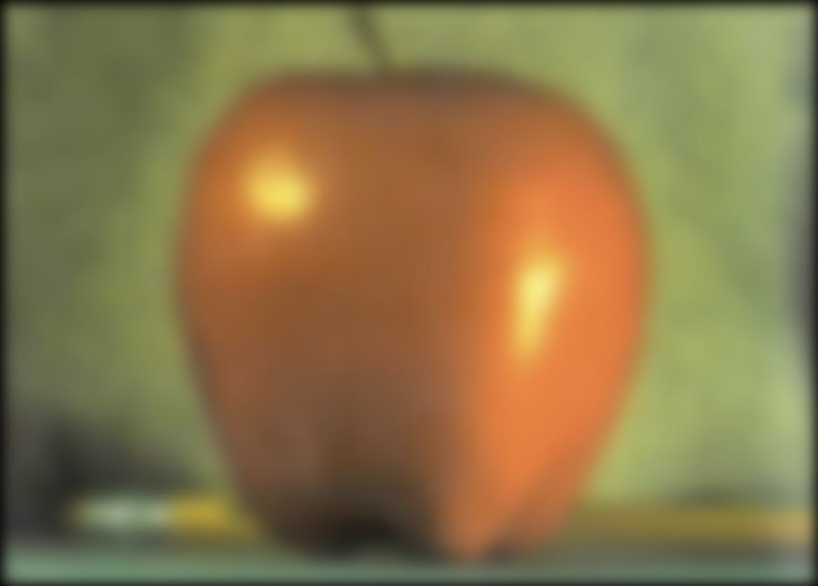
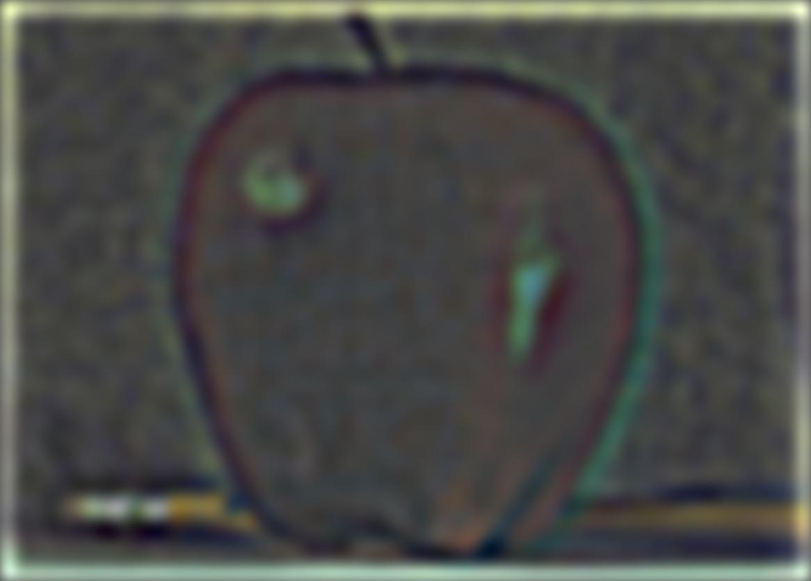

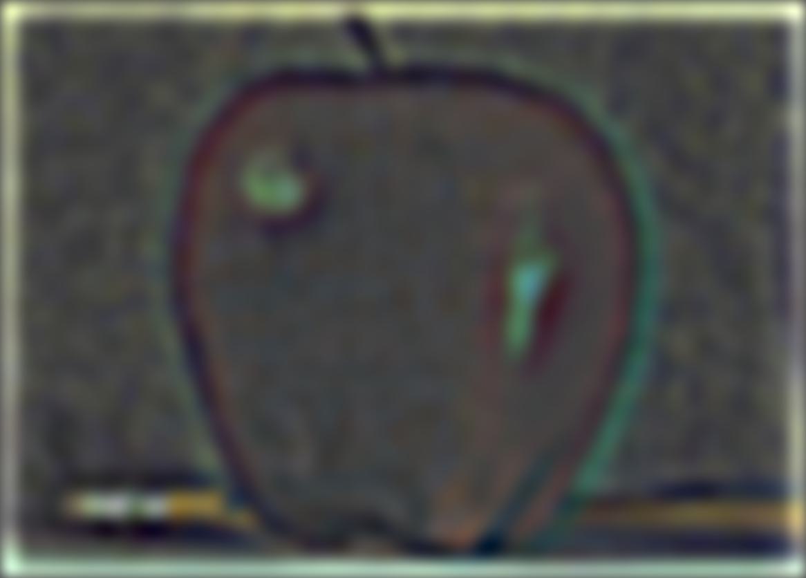

Note that there is one more element in the gaussian stack (as expected given what an element in the laplacian is). Here is the laplacian and guassian for the orange:
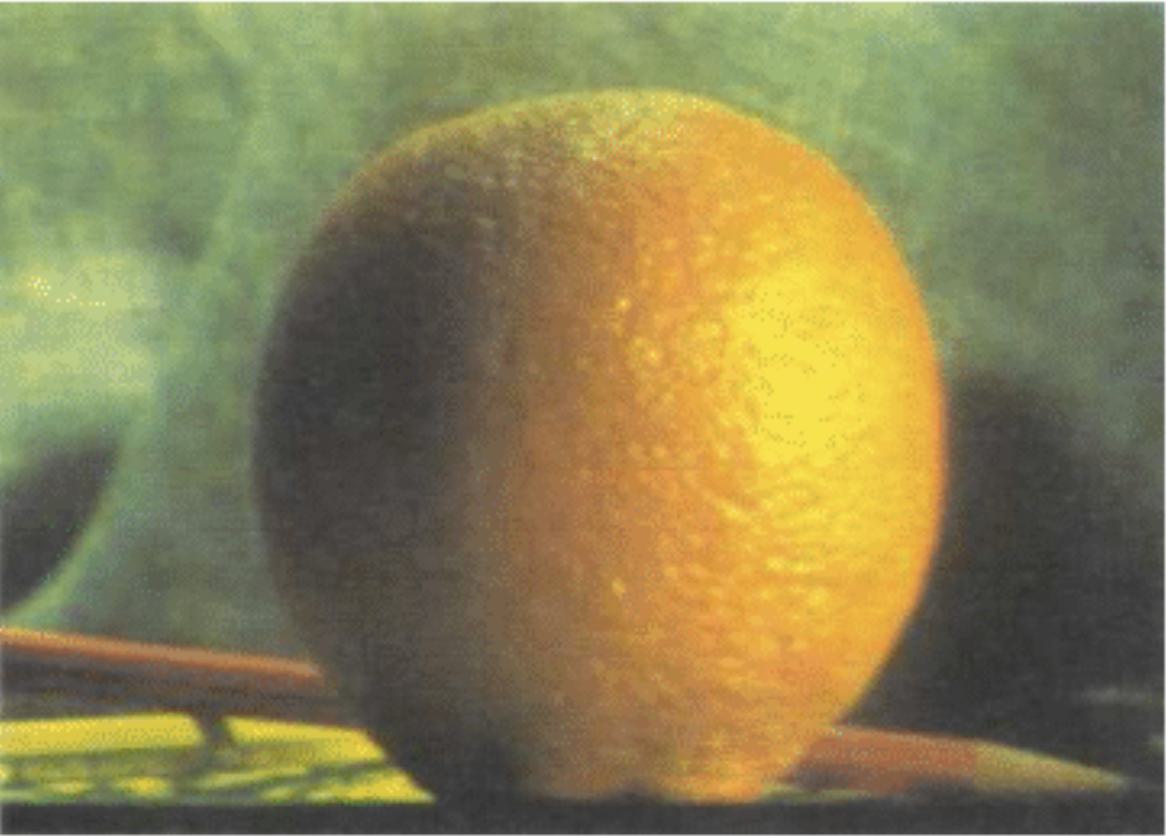
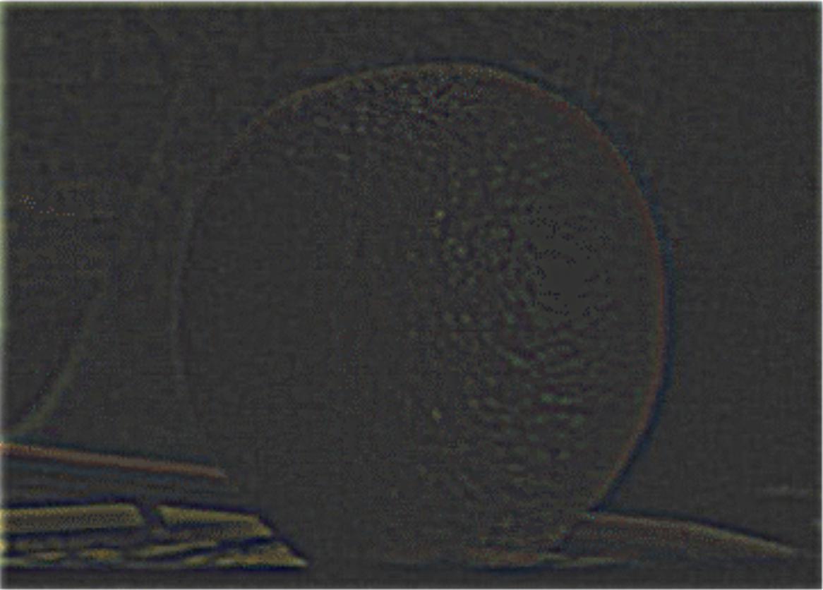


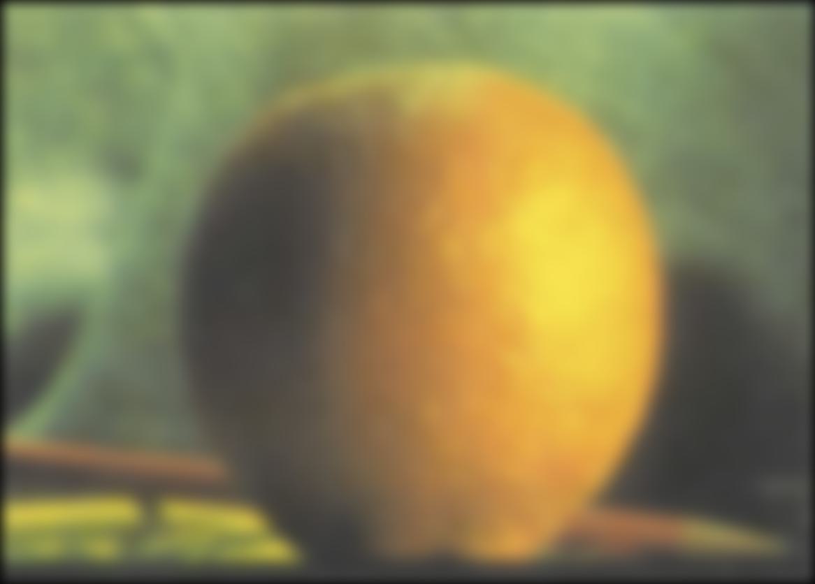
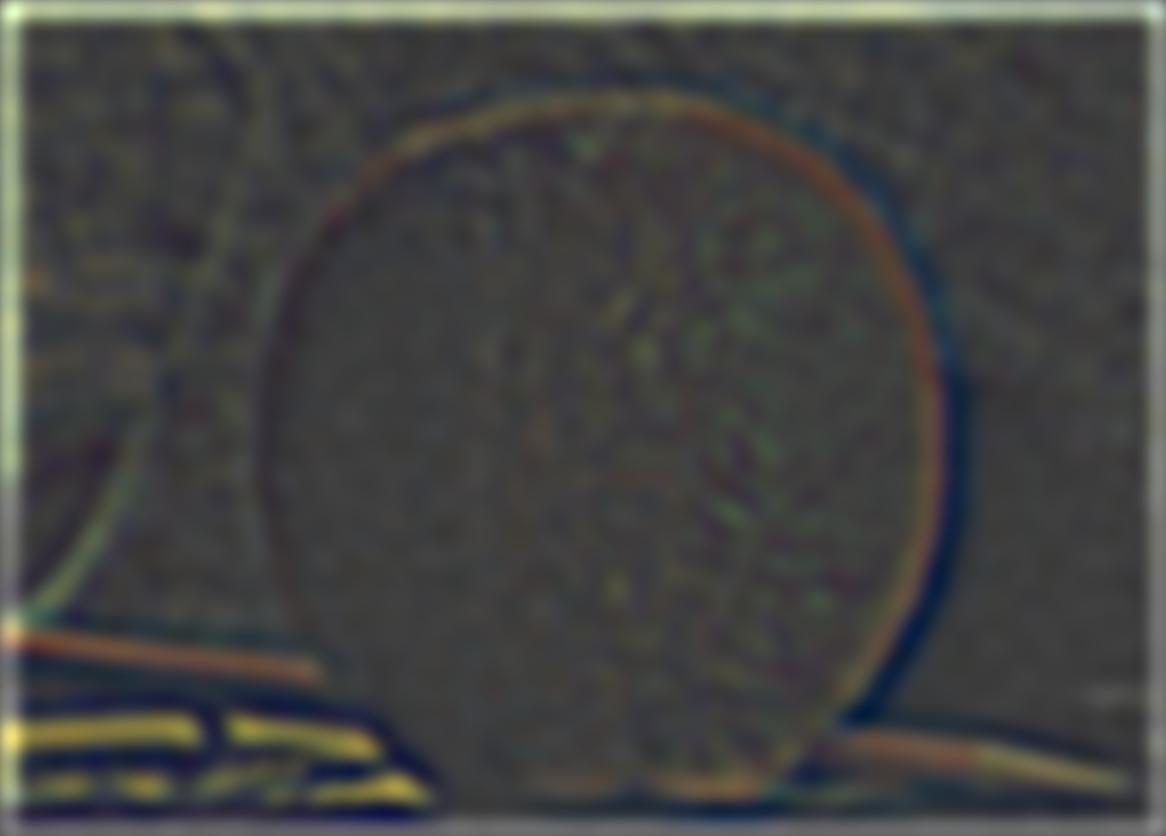
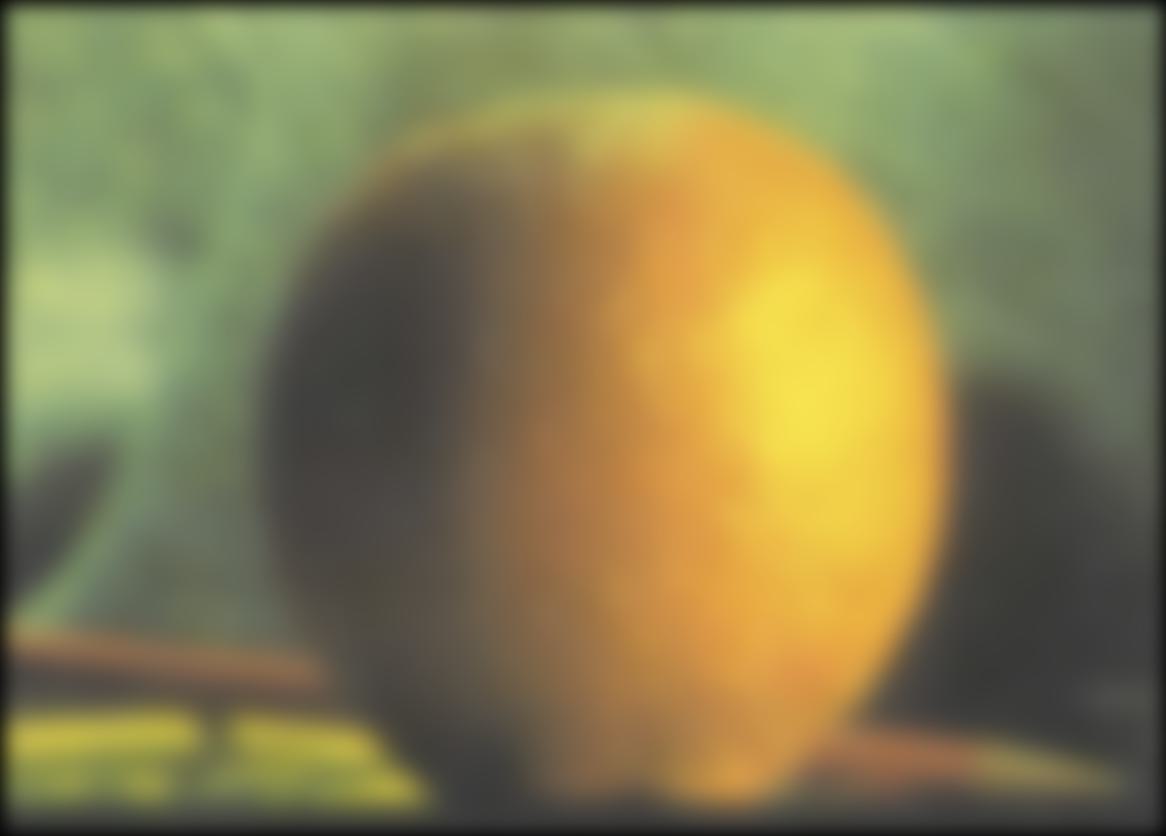
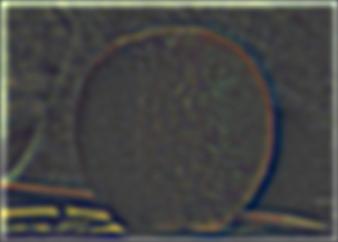

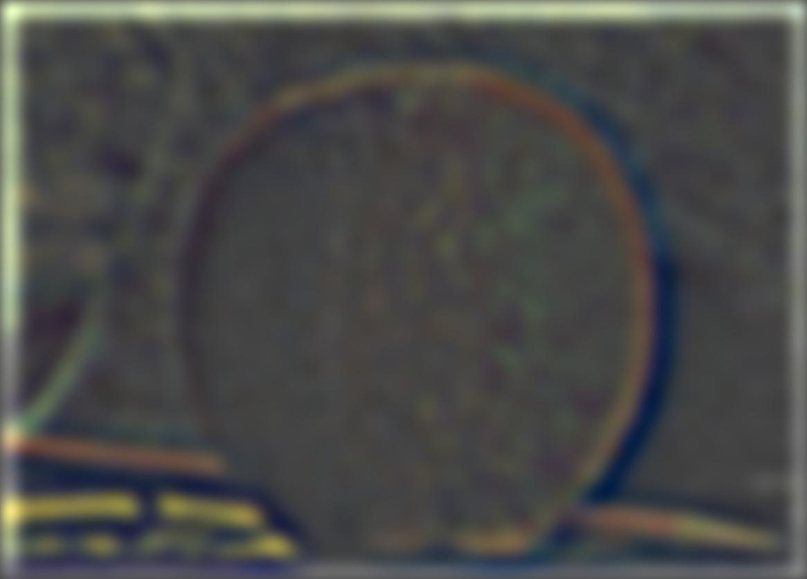
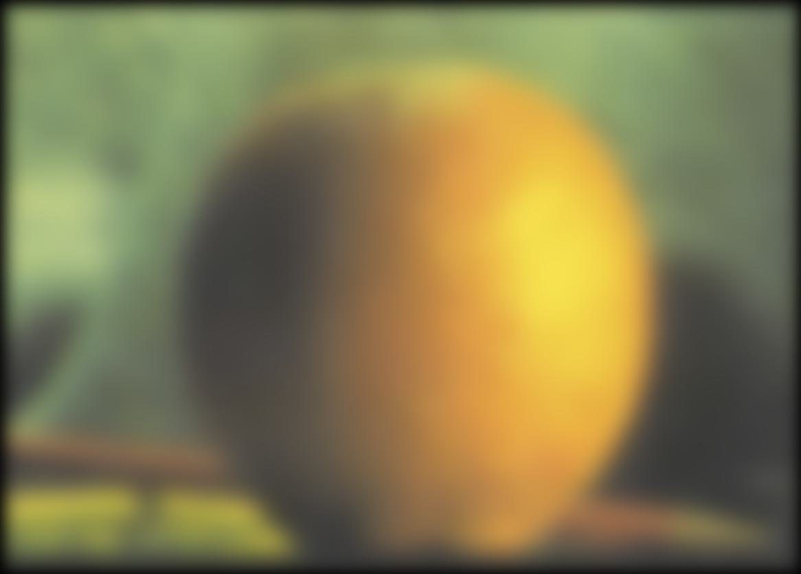
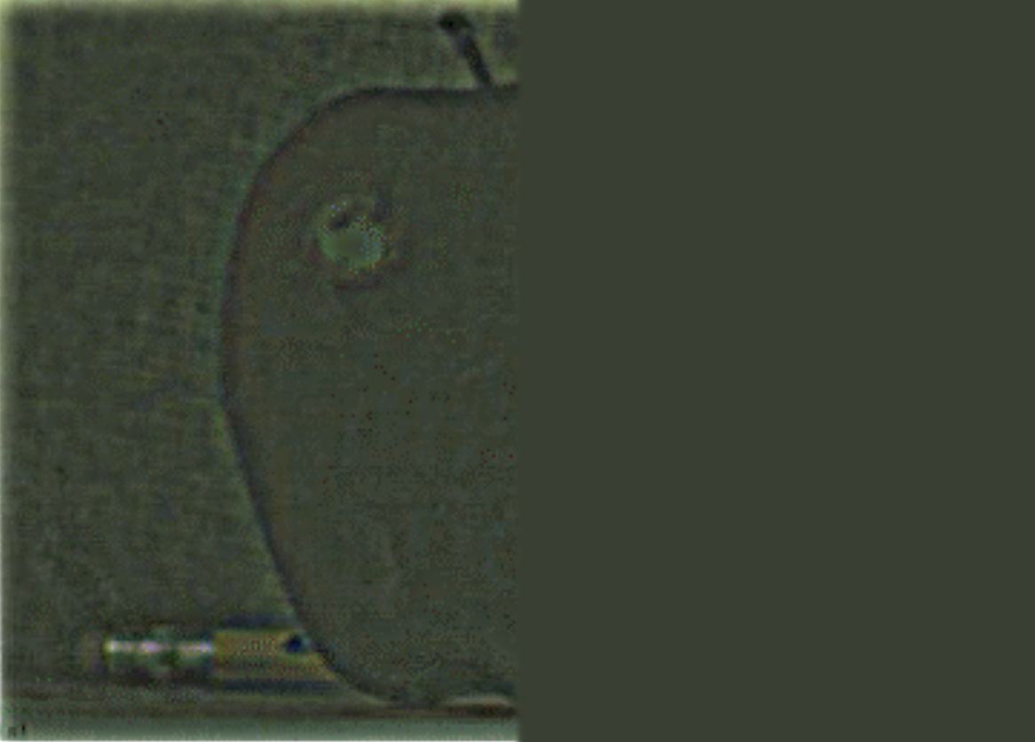
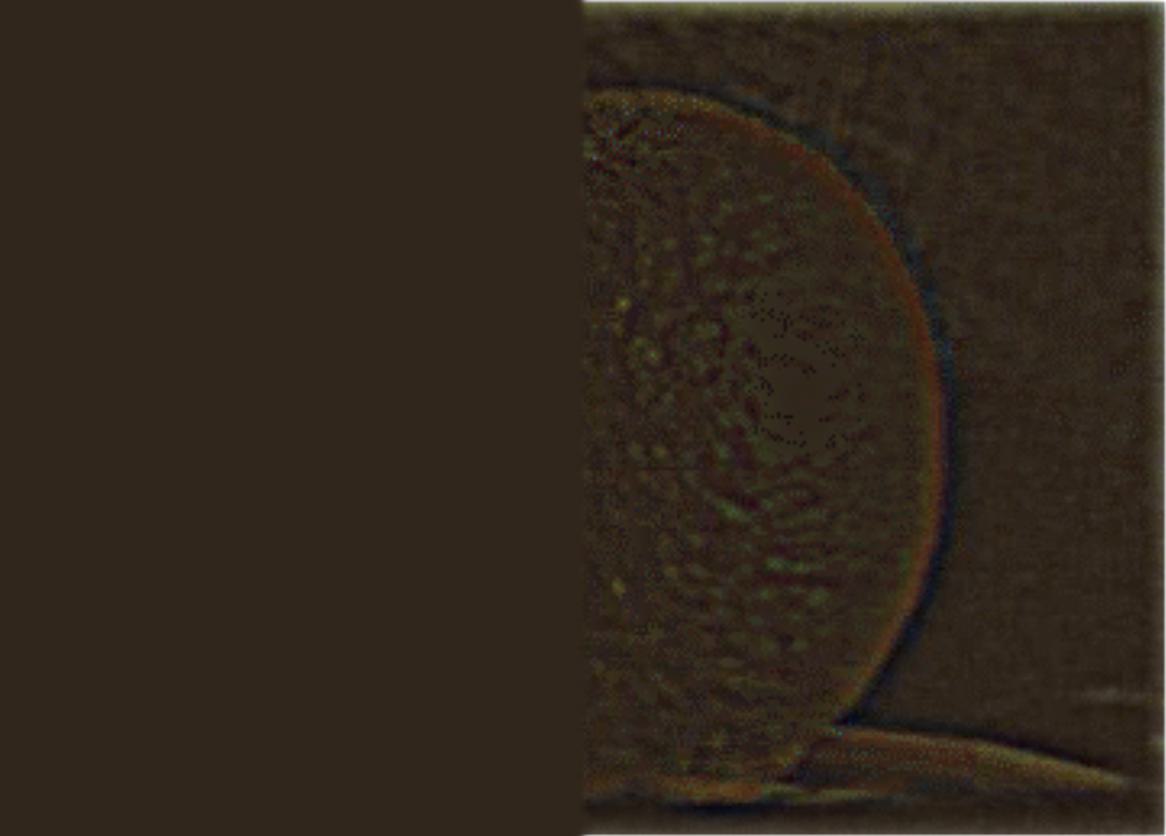
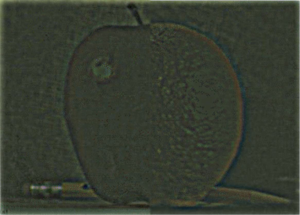
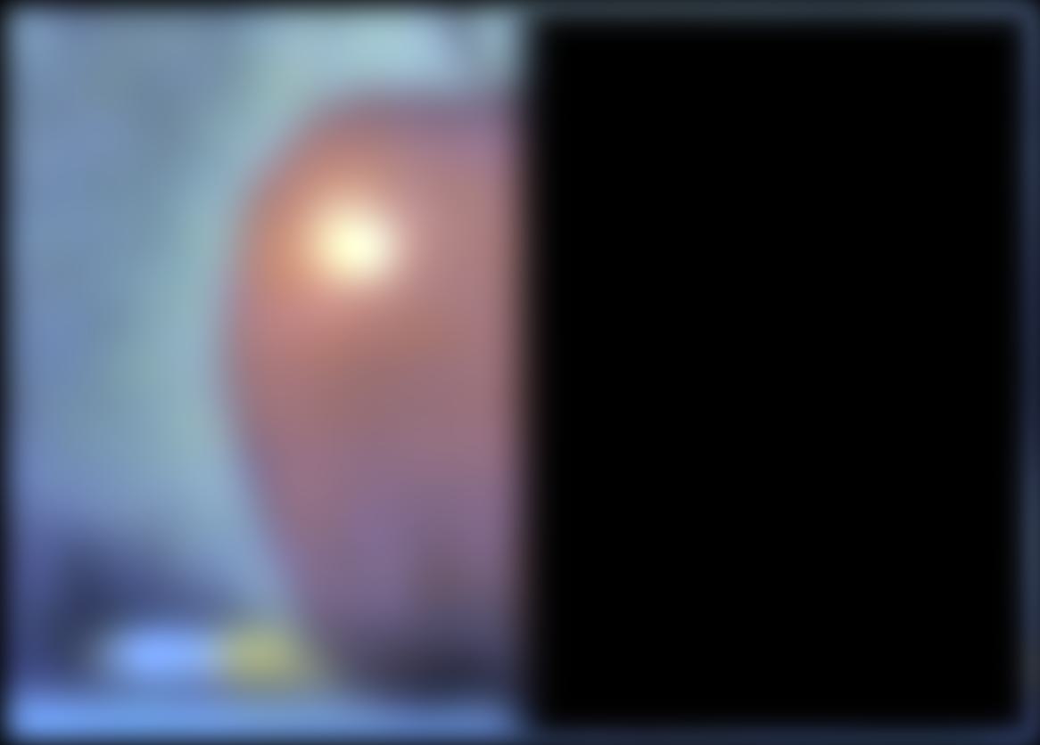
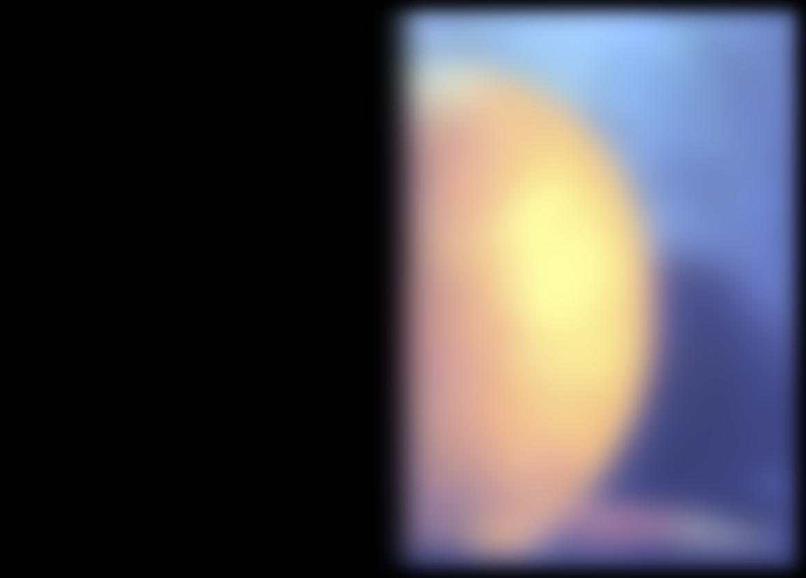
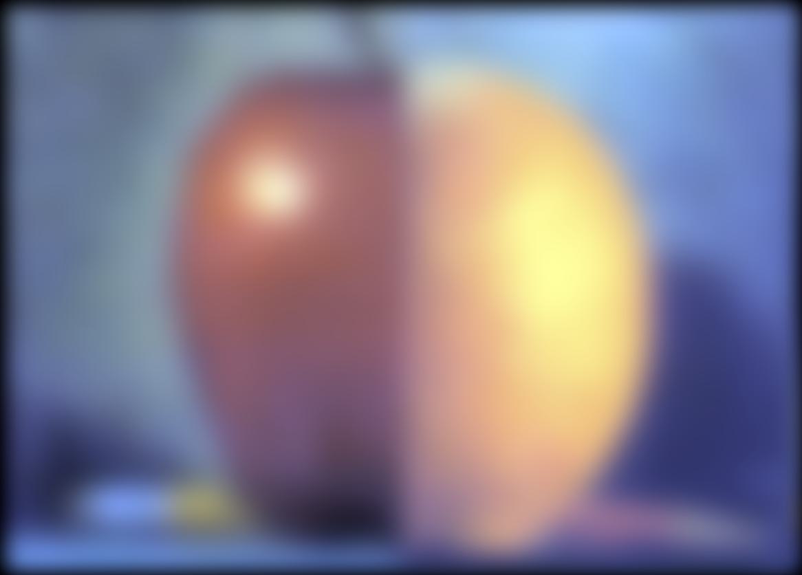
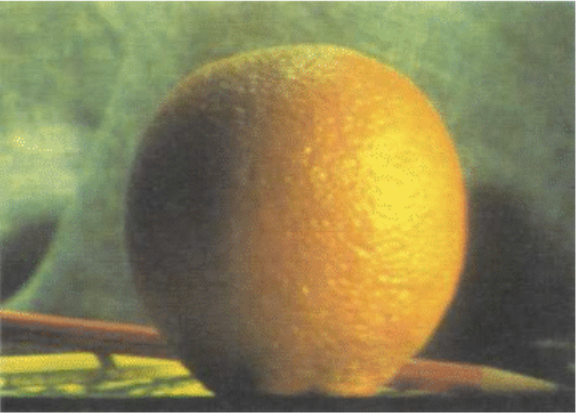
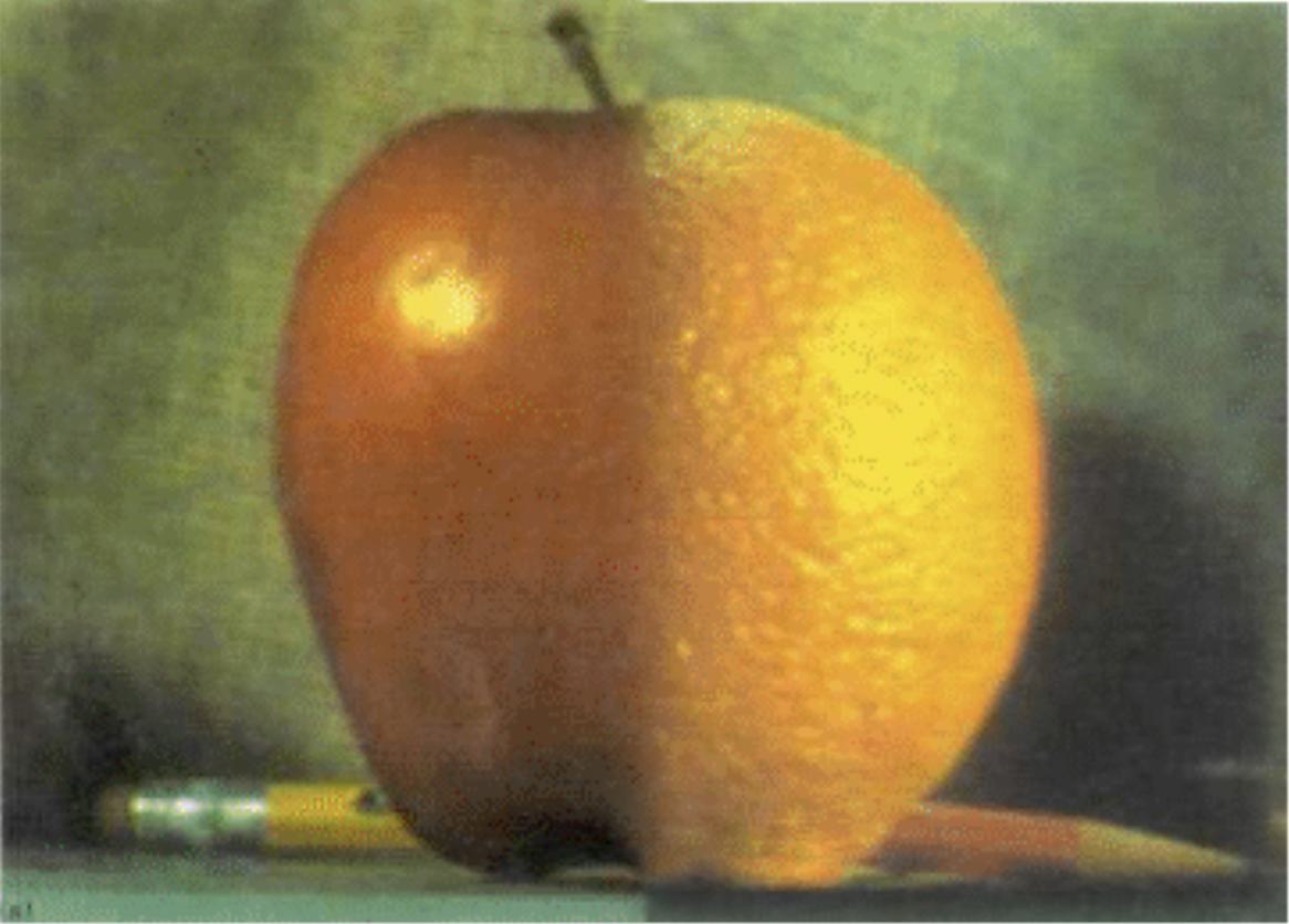
By following the explanations from class and the suggested paper, I learned that Multiresolution blending is achieved masking the laplacian stack of each image at different layers and then sum the results to collapse the image back. For the oraple example:





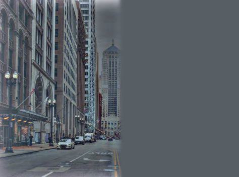
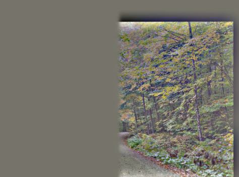
For my own images with a regular mask, I picked to blend landscapes:

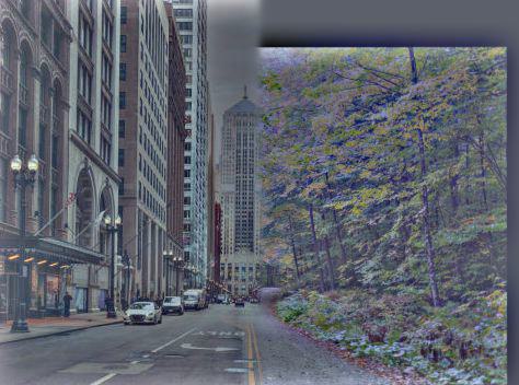

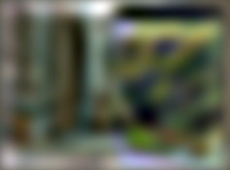
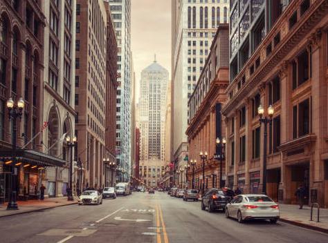
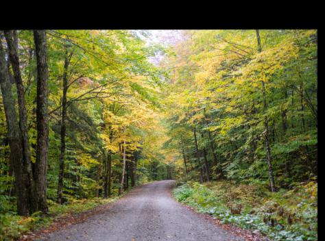
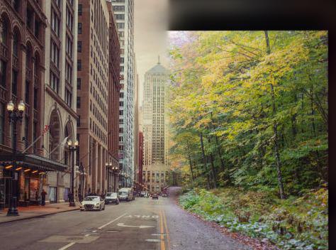
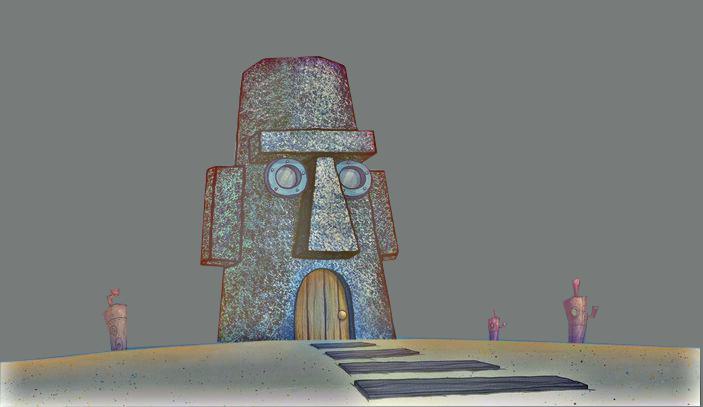
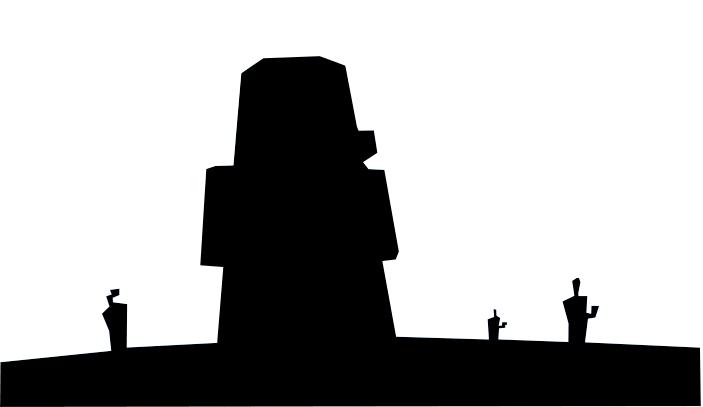
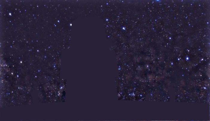
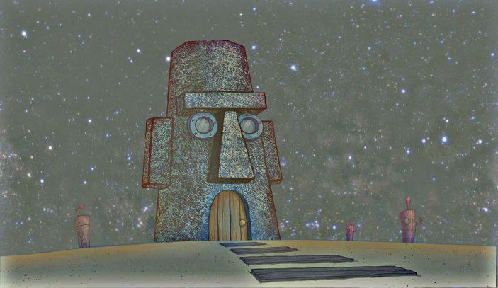
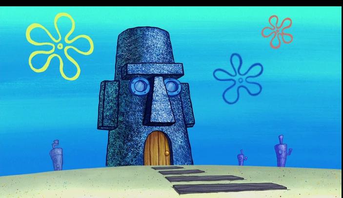
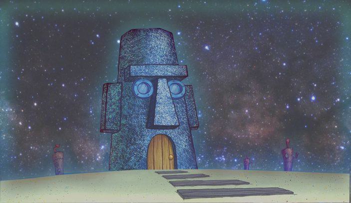
For the irregular mask example, I chose to put squidward's house in space:
