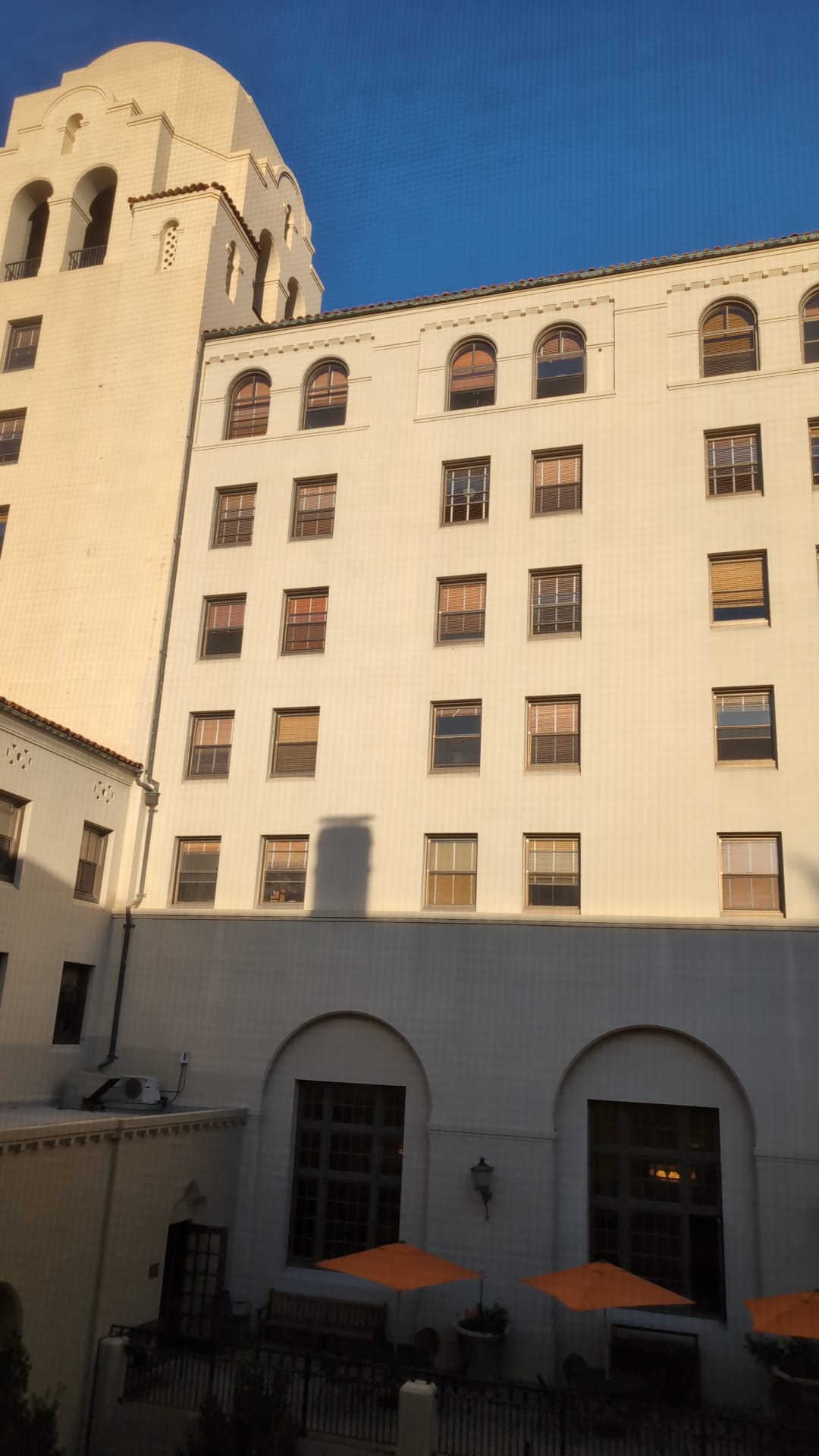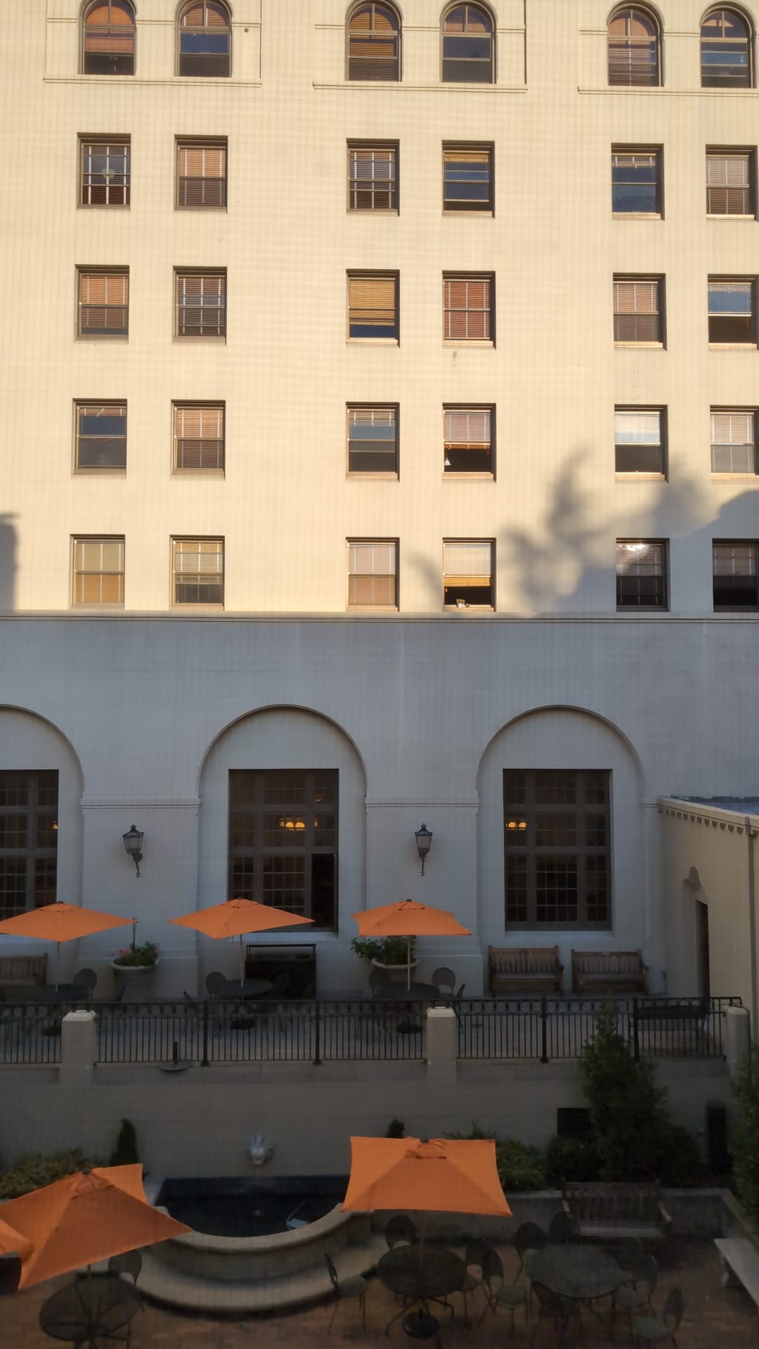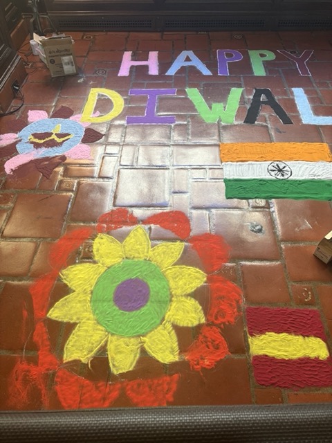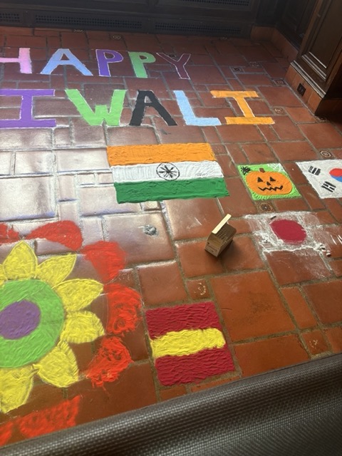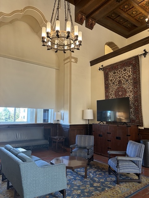
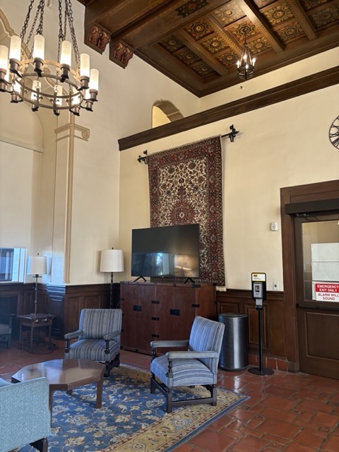
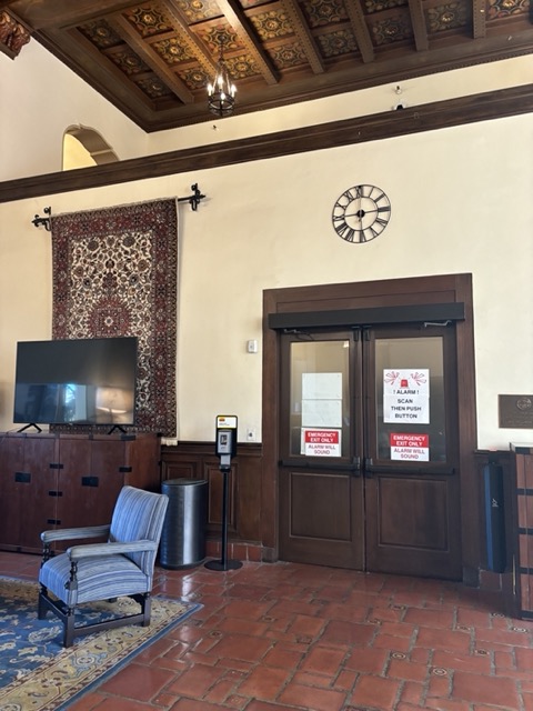
I used these images throughout my project:


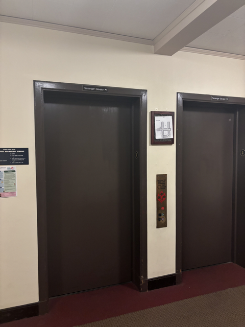
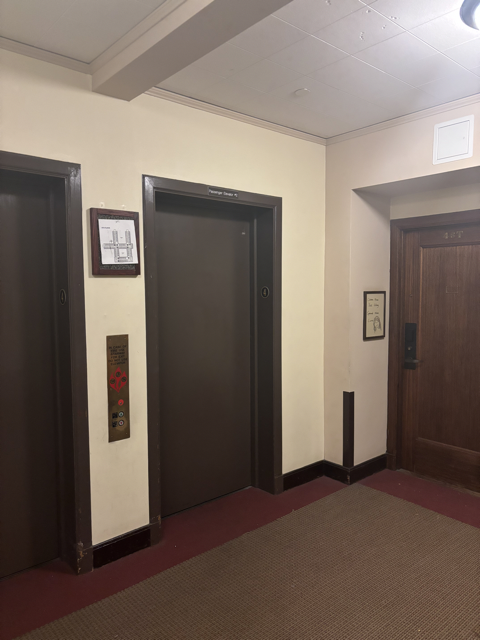
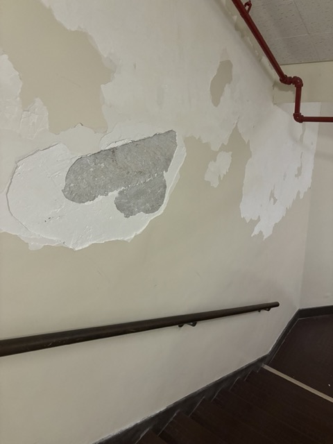
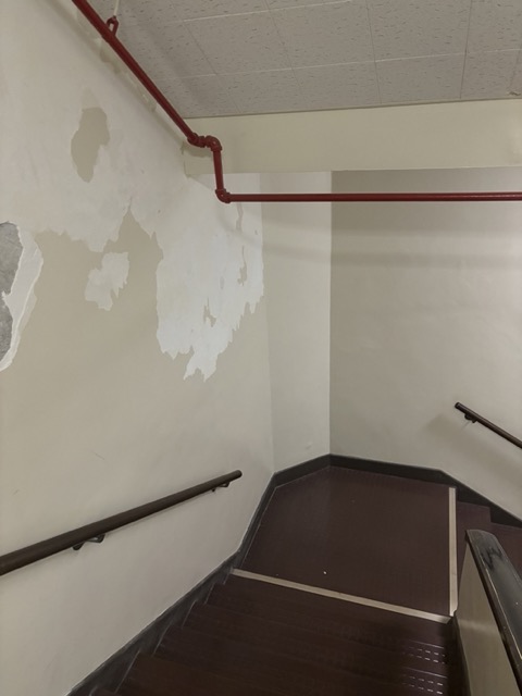
The first step of the project was to define correspondances between the images. To do this, I used the tool from project 3. I observed that for best results, it was preferrable to have a large number of point pairs and have a signiciant overlap between images.
Once I have defined the correspondances, the next task is to recover a transformation such that: \[ \begin{bmatrix} a & b & c \\ d & e & f \\ g & h & 1 \end{bmatrix} \begin{bmatrix} x \\ y \\ 1 \end{bmatrix} = \begin{bmatrix} wx' \\ wy' \\ w \end{bmatrix} \] Note that this transformation won't map points from one image to another directly, but there will also be a scaling component w which we had to account for (it took me some time to realize this). From here, we expand and rearrange to obtain: \[ \begin{bmatrix} x & y & 1 & 0 & 0 & 0 & -xx' & -yx' \\ 0 & 0 & 0 & x & y & 1 & -xy' & -yy' \end{bmatrix} \begin{bmatrix} a \\ b \\ c \\ d \\ e \\ f \\ g \\ h \end{bmatrix} = \begin{bmatrix} x' \\ y' \end{bmatrix} \]
Note that if we pick four points there will be an exact solution to this system. However, in practice, due innacuracy in point selection it is better to select more points and then use least squares.
Once we have recovered the homography H, we can use this matrix to warp one of the image (which is necessary before mosaicing). To do this, I reused some of the techniques from project 3. Specifically, the steps to warp an image are the following:

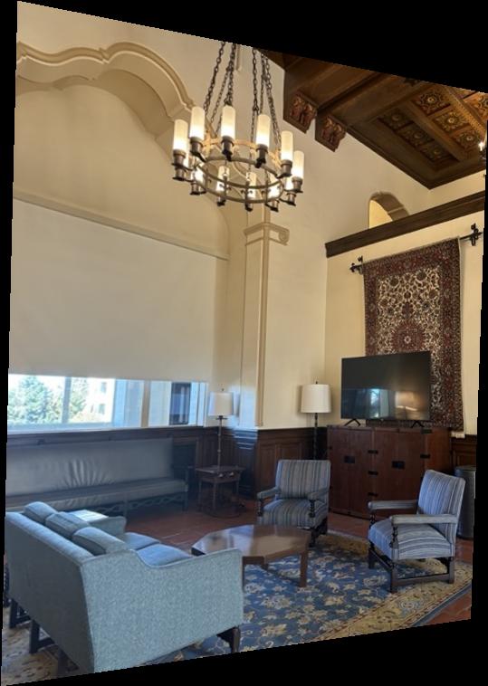

We can get interesting results by warping images that contain rectangular objects in perspective into images that force those objects to appear rectangular. To do this, we simply define a correspondace between the four corners and a rectangle of our choice:
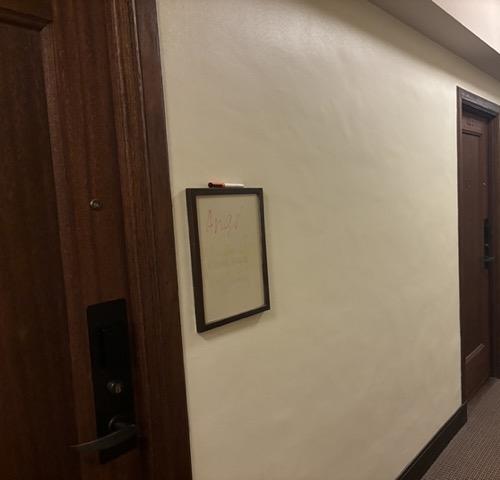
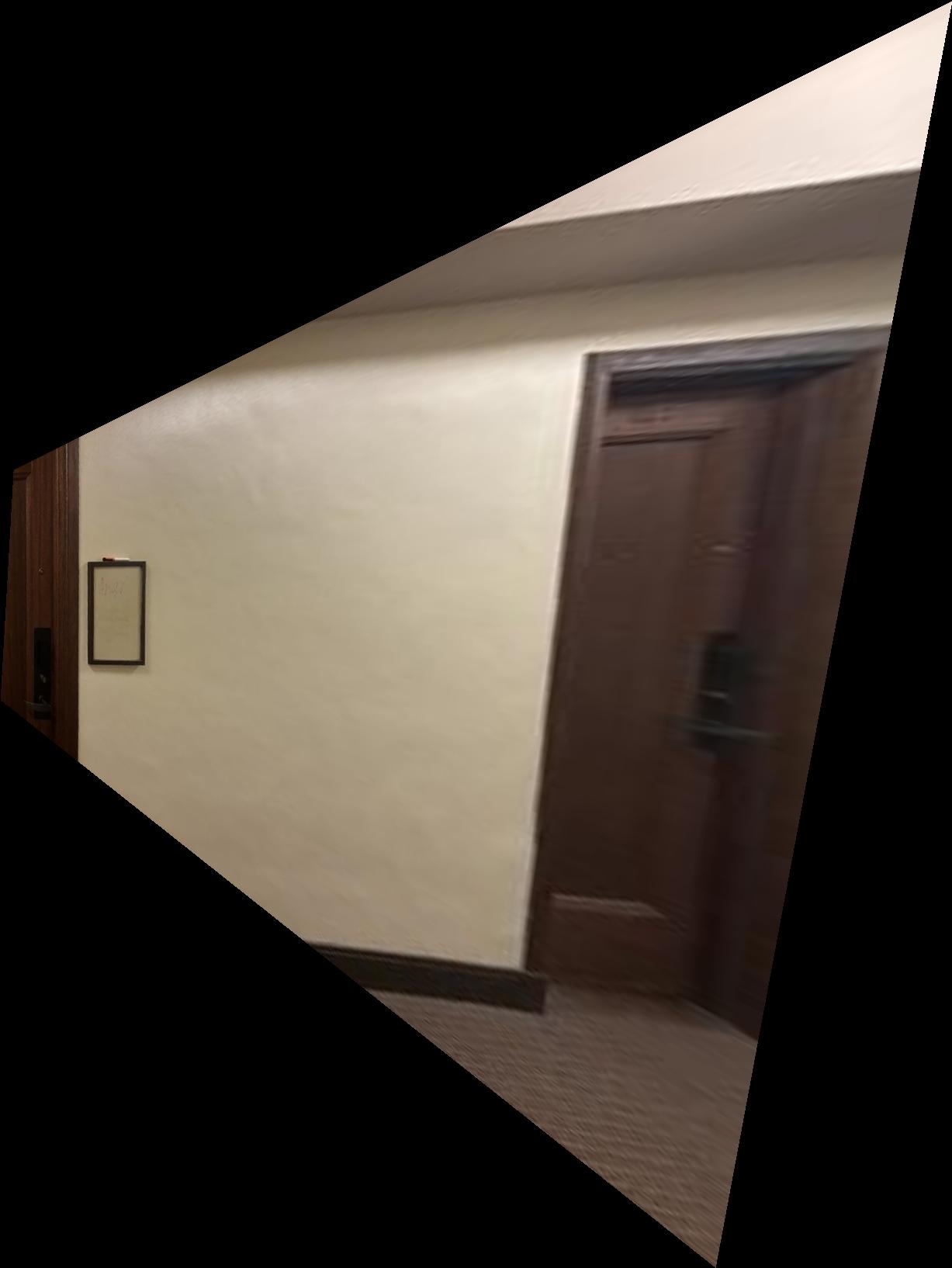
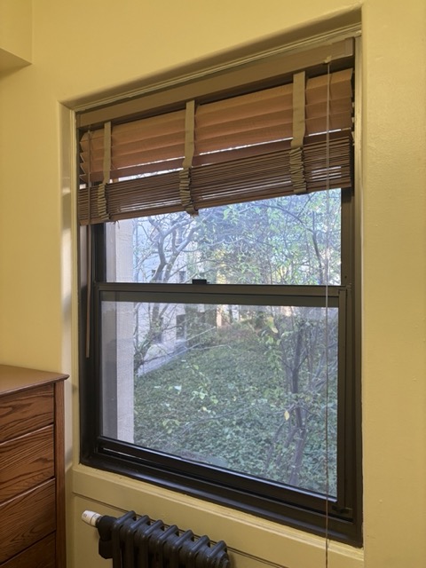
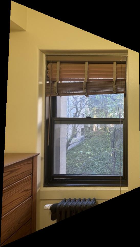
Note that it might seem that the shapes are still not rectangular. I believe that this is a visual effect due to the distorted perspective.
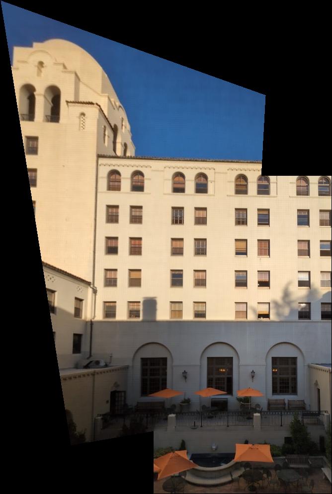
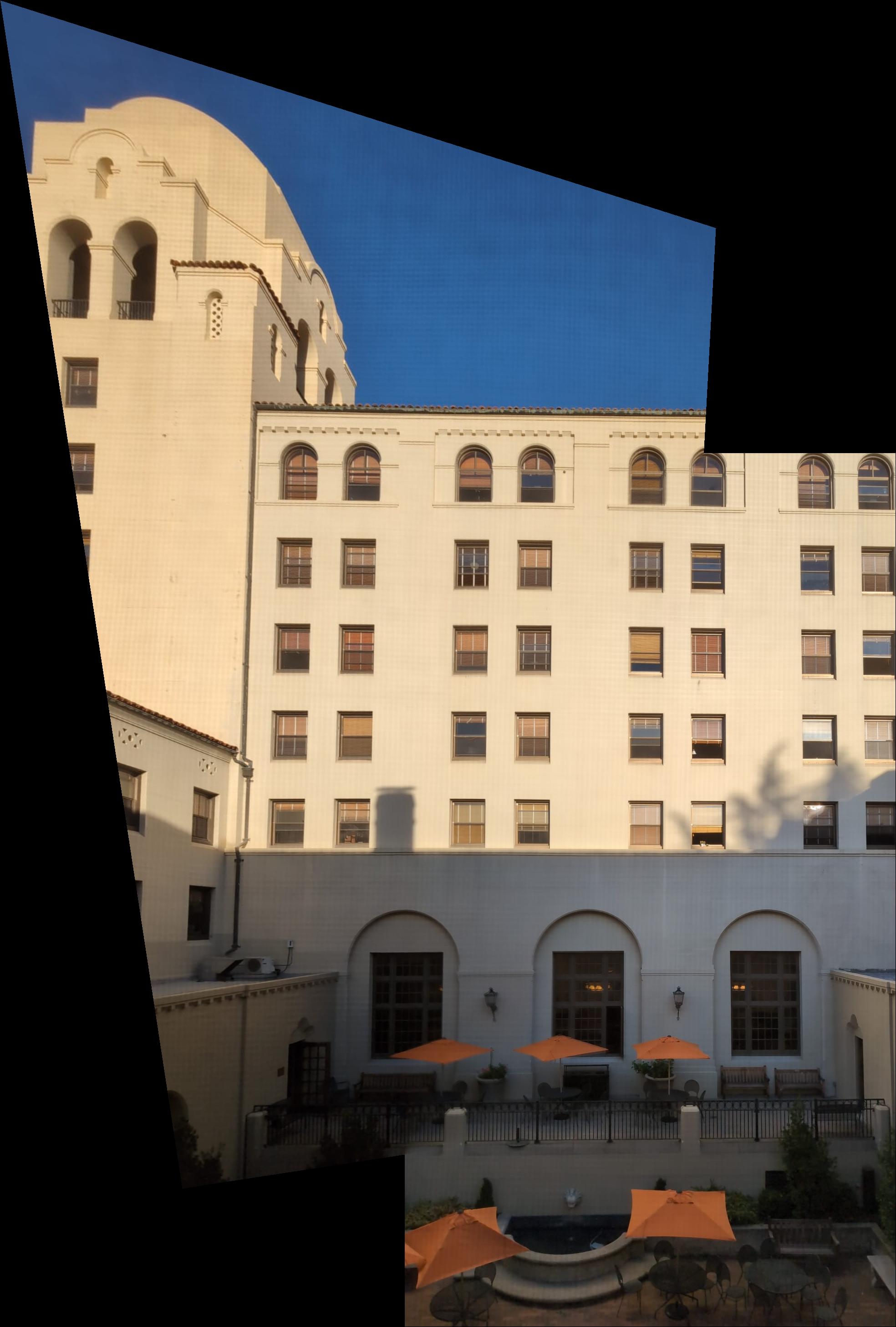
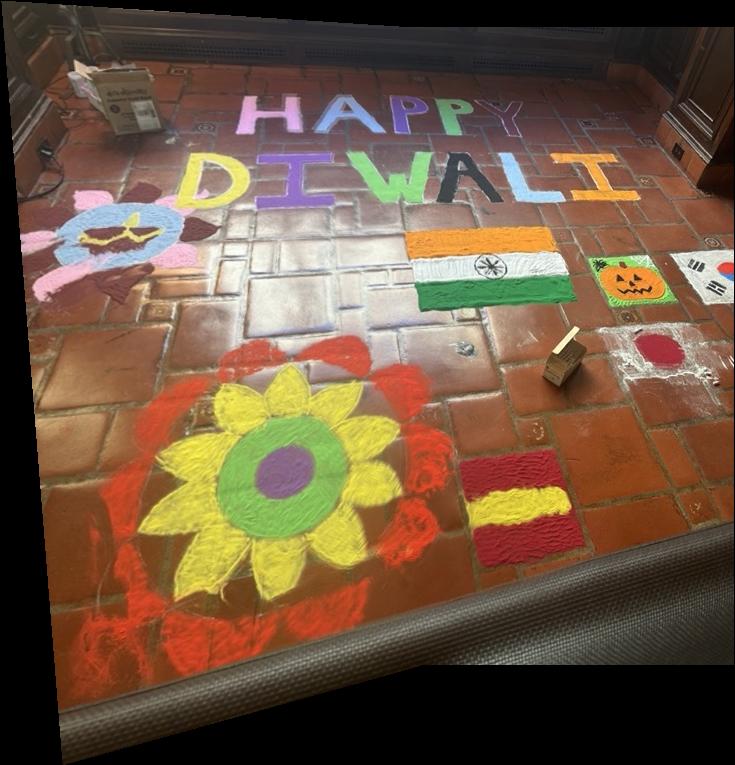
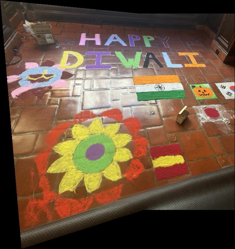
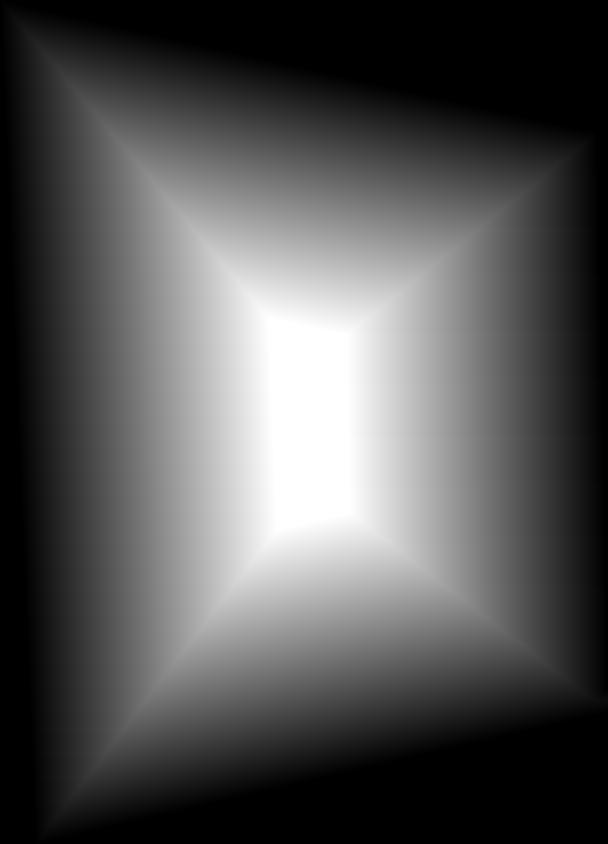
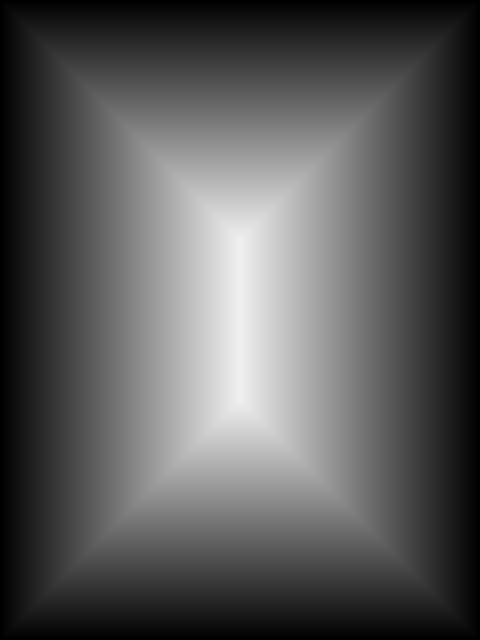
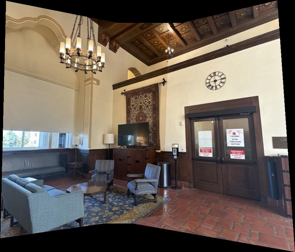
Once we have recovered the homography matrix, we may blend once image into another by superposing the aligned homography with the original destination image. To do this, we start calculating the size of the final projection which is calculated from the sizes of the images and the offset between them. After building the 'canvas' where the result will go, we may superimpose the images. To avoid the appearance of edges between the images, we blend them using an alpha mask than decreases from 0 to 1 between images We obtain the following results:


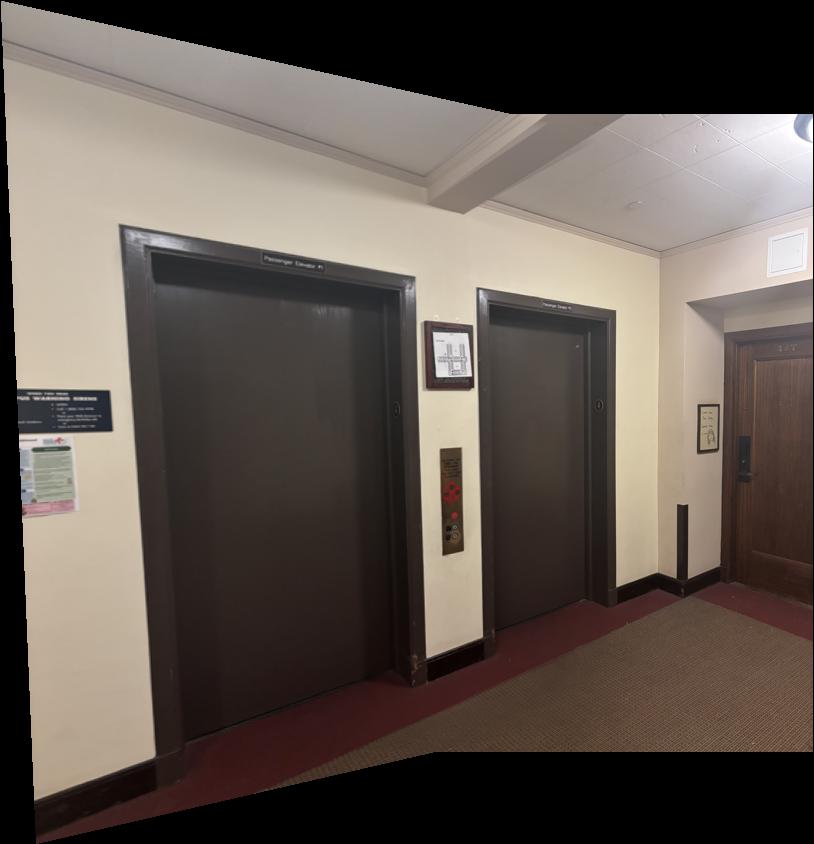
And here are some other mosaics I created:


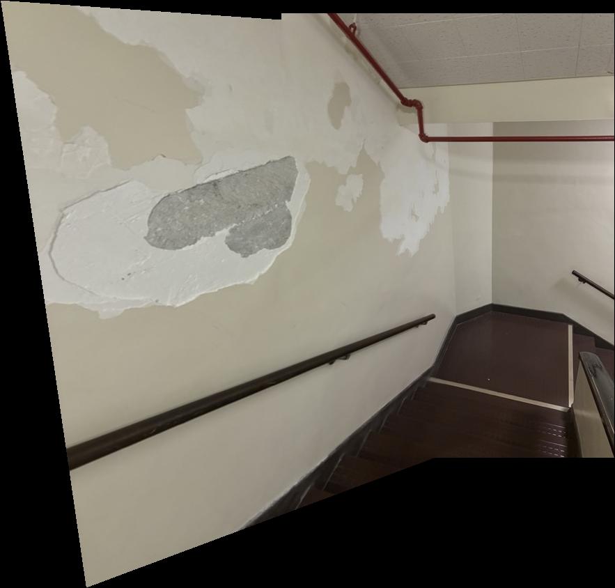


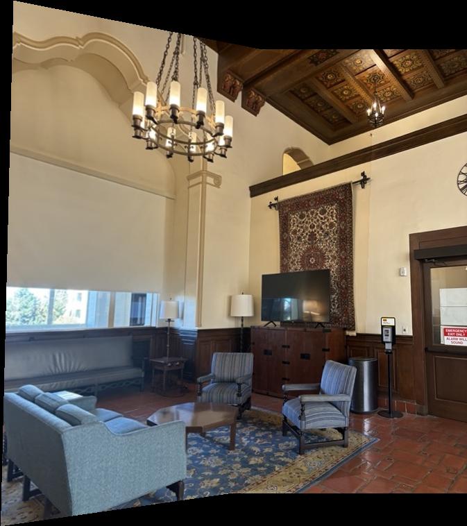
Note that there is no additional difficulty to doing 3 images instead of 2. We obtain the homography between 1 and 3 by multiplying those of 1 and 2 and 2 and 3. I made a naive (not alpha blended) 3 photo mosaic:


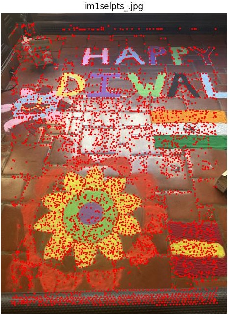
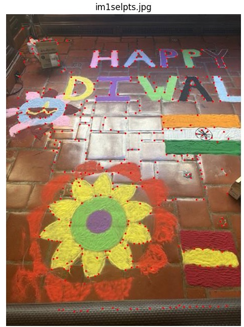
The goal of this section is to eliminate the need for manual correspondance selection. The first step towards achieving this is through corner detection, for which we use the provided harris starter code. Specifically, what the harris algorithm does is calculate a sum of the gradients around an image location and compute its eignevalues. If the matrix indicates sufficient convexity (above a threshold), we'll consider it a corner. In the provided implementation, the threshold is set to a very low value that identifies a lot of potential corners, but to speed up computation and obtain better results I decided to set the threshold a bit higher from the get-go. This is an example output from the harris corner detector:
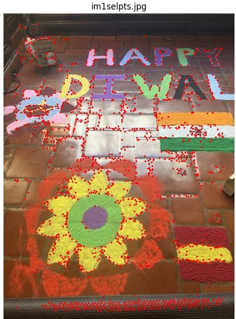
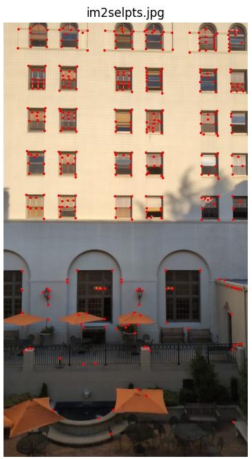
The problem with thresholding directly on the harris value is that we may end up with many points on one section of an image and fewer on a another, yielding suboptimal results. For this reason, we find points that are locally relevant (as opposed to globally significant). I did this by finding the distance from each point to another of greater activation. Then, I kept the k points for which this metric was higher. We should end up with an even spread of corners throughout the image. Here is a nice example:
From the paper, we take the idea to compare downscaled large samples of images around selected corner points rather than naively comparing small patches around the point. This makes the process more stable to slight angle changes between pictures, or similar small errors like that. Also, to avoid aliasing, we first blur the image before extracting features.
Once the features have been extracted, we may compare them to each other. In this case, we apply a simple L2 norm between features to evaluate the likelihood of those two features corresponding to the same image location. Then, I applied Lowe's trick to make outliers less likely (if the first match option is significantly better than the second, then it is likely correct).
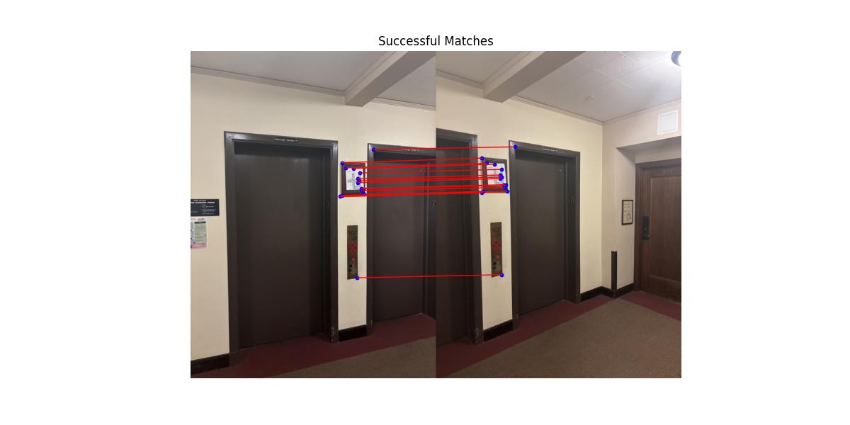
Another feature I implemented is checking for matches in both directions, and applying Lowe's trick both ways. That is to say, if (p1, p2) are to be considered a pair, p1 must be significantly better match than any other for p2 and p2 must be so for p1. I found that, in practice, this almost eliminates outliers completely (I haven't seen any in the images I've tried), thereby eliminating the need for RANSAC. Still, I implemented ransac since its required (more on that later). Here is an example of successful matches between two images:
The final step of the process is to apply RANSAC for robust homography estimation. The goal of RANSAC is to make our homography algorithm robust to outliers which were misidentified in the steps above.
RANSAC works in the following way:


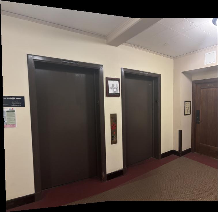
As desired these images are almost identical. For my other examples, I chose different images from section A since I believe I found nicer pictures
